Quickstart doped Tutorial
Tip
You can run this notebook interactively through Google Colab or Binder – just click the links! (Then uncomment the !pip install... cell).
This notebook provides a condensed walkthrough of the core doped workflow for point defect calculations in crystalline materials, going from defect generation → input file writing → parsing → formation energy plotting → thermodynamic analysis.
Each section includes a pointer to the relevant detailed tutorial for more information, and CdTe is used as the example host material throughout.
# # If running on Colab; uncomment to install doped, clone the repo to download the example data and cd in to examples folder:
# !pip install doped
# !git clone https://github.com/SMTG-Bham/doped
# %cd doped/examples
# # Note that when running on Colab, POTCAR file generation will not be possible as this requires the VASP POTCAR directory
# # to be setup with pymatgen (see https://doped.readthedocs.io/en/latest/Installation.html), but all other parts of this
# # notebook can be run directly
1. Defect Generation
The DefectsGenerator class generates the symmetry-inequivalent point defects (vacancies, antisites, and interstitials) for a given host structure, with automatic charge state guessing. See the defect generation tutorial for full details.
from doped.generation import DefectsGenerator

# use the relaxed primitive cell of CdTe (can also load as a pymatgen Structure, and input)
defect_gen = DefectsGenerator("CdTe/relaxed_primitive_POSCAR")
Guessing charge states: 100.0%|██████████| [00:01, 56.87it/s]
Vacancies    Guessed Charges    Conv. Cell Coords    Wyckoff
-----------  -----------------  -------------------  ---------
v_Cd         [+1,0,-1,-2]       [0.000,0.000,0.000]  4a
v_Te         [+2,+1,0,-1]       [0.250,0.250,0.250]  4c

Substitutions    Guessed Charges        Conv. Cell Coords    Wyckoff
---------------  ---------------------  -------------------  ---------
Cd_Te            [+4,+3,+2,+1,0]        [0.250,0.250,0.250]  4c
Te_Cd            [+2,+1,0,-1,-2,-3,-4]  [0.000,0.000,0.000]  4a

Interstitials    Guessed Charges        Conv. Cell Coords    Wyckoff
---------------  ---------------------  -------------------  ---------
Cd_i_C3v         [+2,+1,0]              [0.625,0.625,0.625]  16e
Cd_i_Td_Cd2.83   [+2,+1,0]              [0.750,0.750,0.750]  4d
Cd_i_Td_Te2.83   [+2,+1,0]              [0.500,0.500,0.500]  4b
Te_i_C3v         [+4,+3,+2,+1,0,-1,-2]  [0.625,0.625,0.625]  16e
Te_i_Td_Cd2.83   [+4,+3,+2,+1,0,-1,-2]  [0.750,0.750,0.750]  4d
Te_i_Td_Te2.83   [+4,+3,+2,+1,0,-1,-2]  [0.500,0.500,0.500]  4b

The number in the Wyckoff label is the site multiplicity/degeneracy of that defect in the conventional ('conv.') unit cell, which comprises 4 formula unit(s) of CdTe.
2. Writing Input Files
The DefectsSet class takes a DefectsGenerator (or individual defect entries) and prepares VASP input files for all defect supercell calculations. See the defect generation tutorial for full details.
Automatic input file generation for other codes is planned for future releases.
from doped.vasp import DefectsSet

defect_set = DefectsSet(
    defect_gen,
    user_incar_settings={"ENCUT": 350},  # custom INCAR settings
)

# inspect the generated inputs for one defect:
print(f"INCAR:\n{defect_set.defect_sets['Cd_Te_+2'].vasp_nkred_std.incar}")
INCAR:
# MAY WANT TO CHANGE NCORE, KPAR, AEXX, ENCUT, IBRION, LREAL, NUPDOWN, ISPIN, MAGMOM = Typical variable parameters
AEXX = 0.25
ALGO = Normal  # change to all if zhegv, fexcp/f or zbrent errors encountered, or poor electronic convergence
EDIFF = 1e-05
EDIFFG = -0.01
ENCUT = 350.0
GGA = Pe
HFSCREEN = 0.208
IBRION = 2
ICHARG = 1
ICORELEVEL = 0
ISEARCH = 1
ISIF = 2
ISMEAR = 0
ISPIN = 2
ISYM = 0
KPAR = 4
LASPH = True
LHFCALC = True
LMAXMIX = 4
LORBIT = 11
LREAL = Auto
LVHAR = True
NCORE = 16
NEDOS = 3000
NELECT = 490.0
NKRED = 2
NSW = 200
NUPDOWN = 0.0
PREC = Accurate
PRECFOCK = Fast
SIGMA = 0.05
# cannot be run on Colab: (can't automatically write charged defect INCAR/POTCAR as this
# requires POTCARs to be setup with pymatgen; https://doped.readthedocs.io/en/latest/Installation.html)
defect_set.write_files()  # write all input files to disk
Generating and writing input files: 100%|██████████| 50/50 [00:05<00:00, 9.69it/s]
# # one can write input files (except for POTCARs) on Colab for neutral defects (otherwise
# # POTCAR files needed to specify NELECT (number of electrons) for charged systems):
# defect_set["Cd_Te_0"].write_all(defect_dir="./Cd_Te_0", potcar_spec=True)
!ls Cd_Te_0/*
Cd_Te_+2/vasp_ncl:
Cd_Te_+2.json.gz INCAR            KPOINTS          POTCAR

Cd_Te_+2/vasp_nkred_std:
Cd_Te_+2.json.gz INCAR            KPOINTS          POTCAR

Cd_Te_+2/vasp_std:
Cd_Te_+2.json.gz INCAR            KPOINTS          POTCAR
Tip
Before running the defect supercell relaxations, it is highly recommended to use ShakeNBreak to search for ground-state defect geometries, for which the doped DefectsGenerator can be directly input. This often identifies lower-energy reconstructions that would be missed by a unperturbed local geometry relaxation. See the generation tutorial for details.
3. Parsing Defect Calculations
After running the calculations, DefectsParser automatically identifies the defect type and site from the relaxed structures, computes finite-size charge corrections, and checks calculation settings. See the parsing tutorial for full details.
Here we parse the \(V_{Cd}\) example data on the doped GitHub repository:
from doped.analysis import DefectsParser

dielectric = 9.13  # isotropic dielectric constant of CdTe, use tensor/array for anisotropic
dp = DefectsParser("CdTe/v_Cd_example_data", dielectric=dielectric)
Parsed v_Cd_0/vasp_ncl: 100%|██████████| 3/3 [00:20<00:00,  6.84s/it]
analysis.py:1986: UserWarning: Defects v_Cd_0 have been detected to have dimer bonds:
{'Te': {'Te(37)': {'Te(55)': '2.75 A'}}}
which often adopt multiplet spin states (e.g. triplet O2, Si dimers etc, see https://doped.readthedocs.io/en/latest/Tips.html#magnetization). You may want to test setting `NUPDOWN` to 2 / 3 (for even / odd charge states) or higher for this defect. You can control this warning with the ``rtol`` kwarg.
for name, defect_entry in dp.defect_dict.items():
    print(f"{name}:")
    if defect_entry.charge_state != 0:
        print(f"  Charge = {defect_entry.charge_state:+}, "
              f"charge correction: {list(defect_entry.corrections.values())[0]:+.3f} eV")
    print(f"  Relaxed site: {defect_entry.defect_supercell_site.frac_coords.round(3)}\n")
v_Cd_0:
  Relaxed site: [0.5 0.5 0.5]

v_Cd_-1:
  Charge = -1, charge correction: +0.225 eV
  Relaxed site: [0. 0. 0.]

v_Cd_-2:
  Charge = -2, charge correction: +0.739 eV
  Relaxed site: [0. 0. 0.]
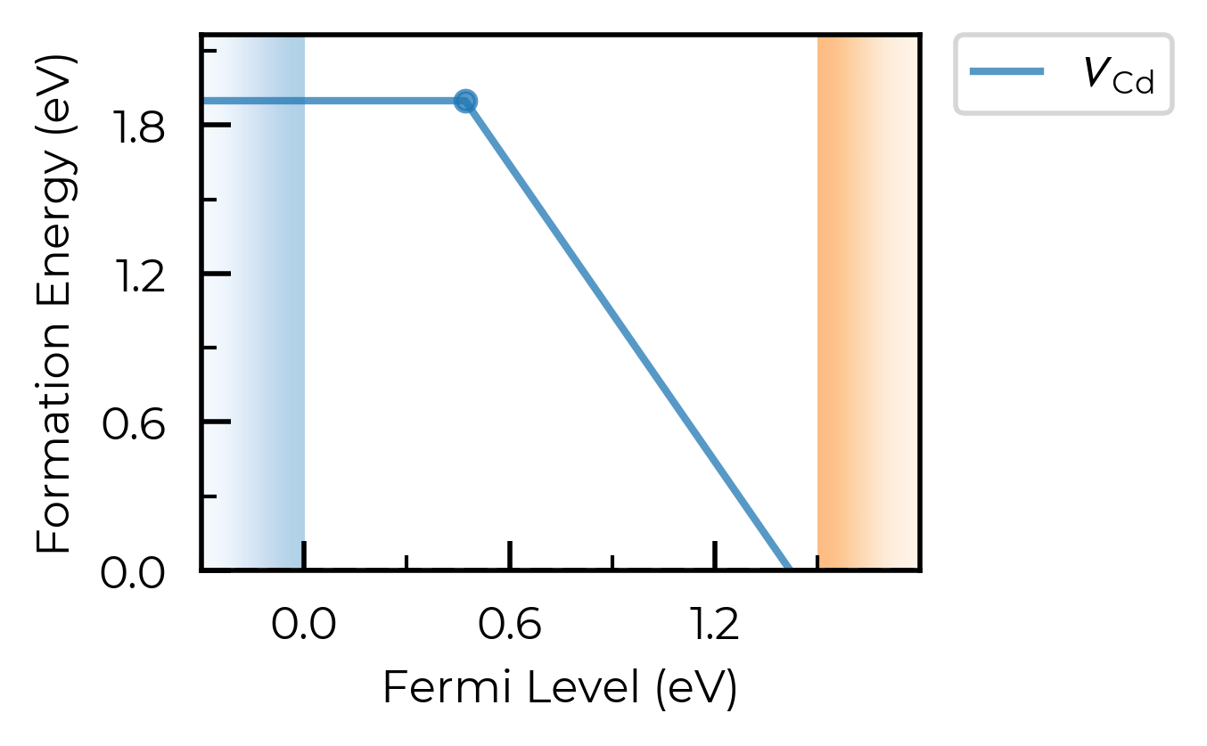
4. Formation Energy Diagram
The transition level diagram (TLD) shows defect formation energies as a function of the Fermi level. This is the central plot for analysing defect behaviour. See the thermodynamics tutorial and plotting customisation tutorial for more options.
To plot formation energy diagrams, and perform a range of other (thermodynamic) analyses, we use the DefectThermodynamics class.
v_Cd_thermo = dp.get_defect_thermodynamics()  # get the DefectThermodynamics object
v_Cd_thermo.get_symmetries_and_degeneracies()
| Site_Symm | Defect_Symm | g_Orient | g_Spin | g_Total | Mult | ||
|---|---|---|---|---|---|---|---|
| Defect | q | ||||||
| v_Cd | 0 | Td | C2v | 6.0 | 1.0 | 6.0 | 1.0 |
| -1 | Td | C3v | 4.0 | 2.0 | 8.0 | 1.0 | |
| -2 | Td | Td | 1.0 | 1.0 | 1.0 | 1.0 |
To obtain the formation energies, we need to set the chemical potentials of the host and any dopant/extrinsic species. To determine the chemical potential limits, we need to compute the energies of competing secondary phases, as shown in the chemical potentials tutorial (using CompetingPhases and CompetingPhasesAnalyzer). Here we will load our pre-computed chemical potential limits for CdTe:
from monty.serialization import loadfn

CdTe_chempots = loadfn("CdTe/CdTe_chempots.json")  # chemical potential limits
v_Cd_thermo.chempots = CdTe_chempots  # set chemical potentials for subsequent analyses
formation_energy_plot = v_Cd_thermo.plot(limit="Te-rich")
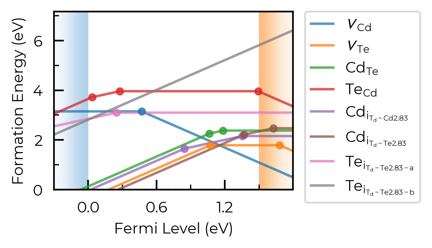
Loading the full CdTe defect thermodynamics
For the rest of this tutorial, we load a pre-parsed DefectThermodynamics object containing all intrinsic CdTe point defects (vacancies, antisites and interstitials):
from monty.serialization import loadfn

CdTe_thermo = loadfn("CdTe/CdTe_thermo_wout_meta.json.gz")  # DefectThermodynamics object
CdTe_thermo.chempots = CdTe_chempots  # set chemical potentials for subsequent analyses
CdTe_thermo.plot(limit="Cd-rich")
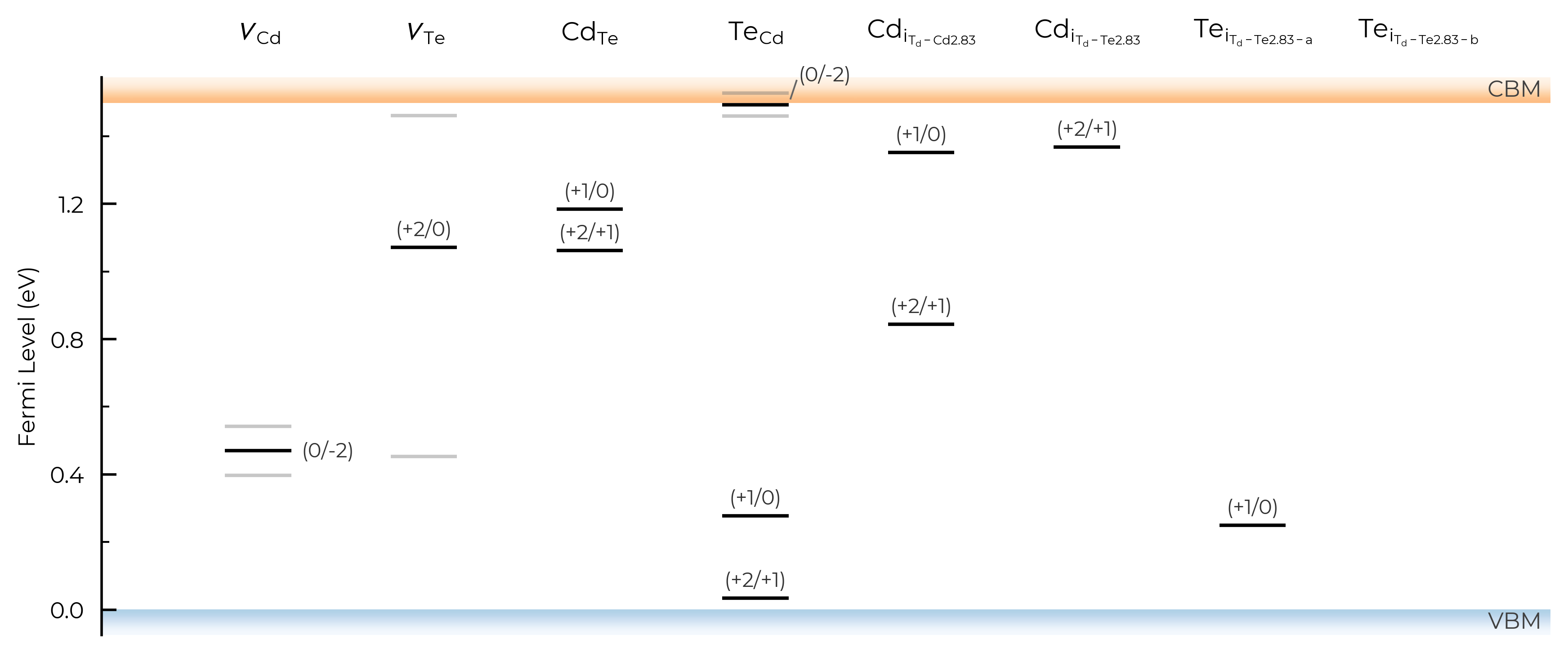
We can also plot the defect charge transition levels on a vertical energy level diagram:
CdTe_thermo.plot_transition_levels()
6. Thermodynamic Analysis
Equilibrium Fermi Level & Carrier Concentrations
We can solve for the equilibrium Fermi level (at which charge neutrality is satisfied) and get the corresponding defect and carrier concentrations, using get_fermi_level_and_concentrations(). This requires the bulk electronic density of states (DOS):
vasprun_path = "CdTe/CdTe_prim_k181818_NKRED_2_vasprun.xml.gz"  # bulk DOS calculation

fermi_level, electrons, holes, conc_df = CdTe_thermo.get_fermi_level_and_concentrations(
    bulk_dos=vasprun_path, limit="Te-rich",
    annealing_temperature=900, quenched_temperature=300,  # annealed at 900K, quenched to RT
)  # using frozen defect approximation
print(f"Equilibrium Fermi level: {fermi_level:.3f} eV above VBM")
print(f"Electron concentration:  {electrons:.1e} cm⁻³")
print(f"Hole concentration:      {holes:.1e} cm⁻³")
Equilibrium Fermi level: 0.398 eV above VBM
Electron concentration:  2.6e-02 cm⁻³
Hole concentration:      2.1e+12 cm⁻³
conc_df.head() # concentration DataFrame
| Concentration (cm^-3) | Formation Energy (eV) | Charge State Population | Total Concentration (cm^-3) | ||
|---|---|---|---|---|---|
| Defect | Charge | ||||
| v_Cd | 0 | 1.464e+15 | 1.899 | 99.44% | 1.472e+15 |
| -1 | 7.254e+12 | 2.043 | 0.49% | 1.472e+15 | |
| -2 | 9.380e+11 | 2.042 | 0.06% | 1.472e+15 | |
| v_Te | +2 | 1.789e+08 | 1.692 | 100.00% | 1.789e+08 |
| +1 | 7.349e-14 | 2.983 | 0.00% | 1.789e+08 |
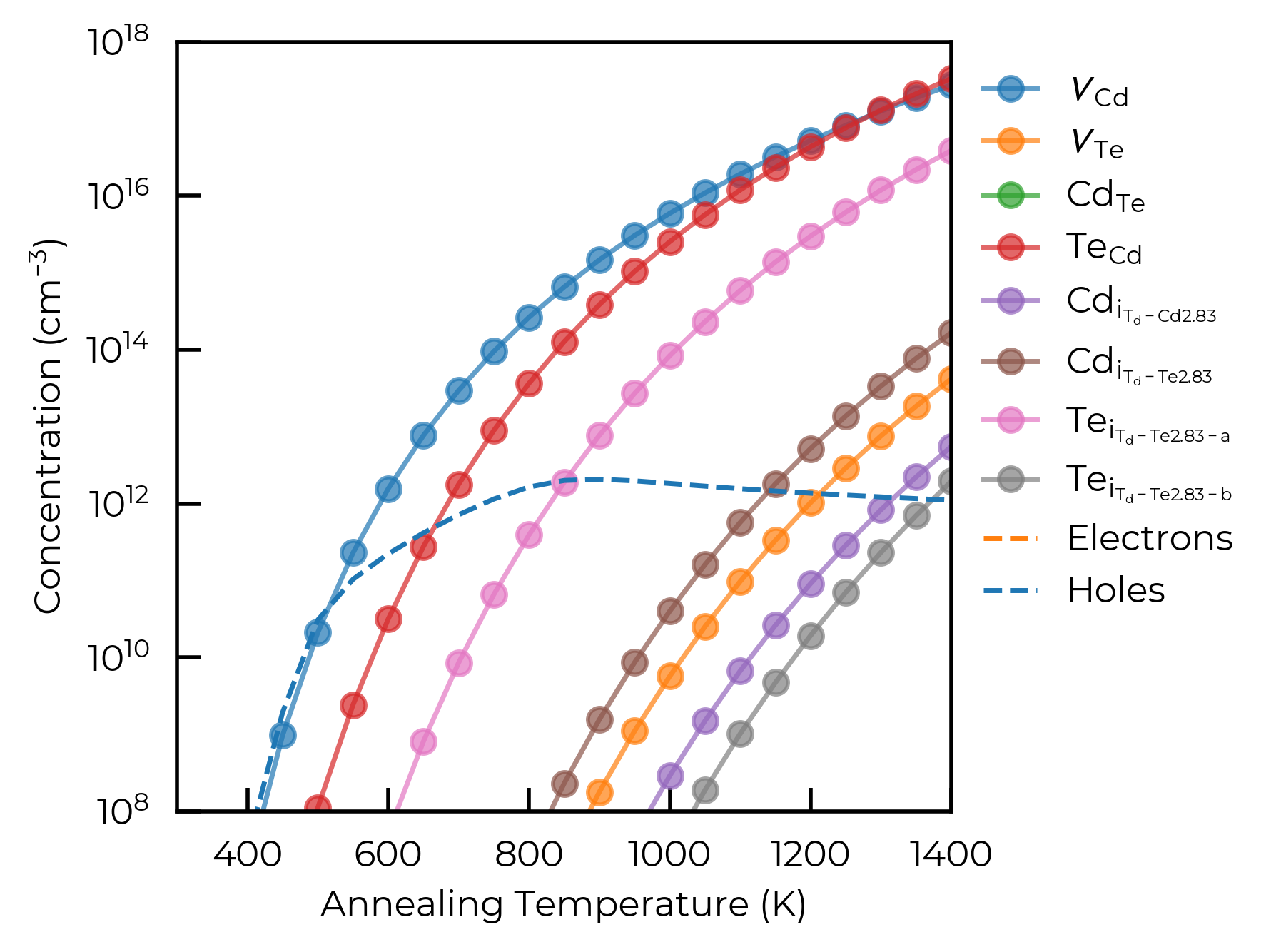
Concentration vs Temperature (FermiSolver)
The FermiSolver class provides powerful tools for scanning defect and carrier concentrations over temperatures, chemical potentials and more. See the FermiSolver tutorial for full details.
from doped.thermodynamics import FermiSolver

fs = FermiSolver(defect_thermodynamics=CdTe_thermo, bulk_dos=vasprun_path)
For example, scanning over annealing temperatures for the Te-rich chemical potential limit with scan_temperature():
import matplotlib.pyplot as plt
import doped
from doped.utils.plotting import format_defect_name

plt.style.use(f"{doped.__path__[0]}/utils/doped.mplstyle")

temperatures = range(300, 1410, 50)
temp_df = fs.scan_temperature(
    limit="Te-rich", annealing_temperature_range=temperatures, per_charge=False
)  # per_charge=False gives total concentrations per defect species

fig, ax = plt.subplots()
for defect in temp_df.index.unique():
    defect_df = temp_df.loc[defect]
    ax.plot(
        defect_df["Annealing Temperature (K)"],
        defect_df["Concentration (cm^-3)"],
        label=format_defect_name(defect, include_site_info=True, wout_charge=True),
        marker="o", alpha=0.7,
    )

# also plot carrier concentrations
first_defect_df = temp_df.loc[temp_df.index.unique()[0]]
ax.plot(first_defect_df["Annealing Temperature (K)"], first_defect_df["Electrons (cm^-3)"],
        ls="--", color="C1", label="Electrons")
ax.plot(first_defect_df["Annealing Temperature (K)"], first_defect_df["Holes (cm^-3)"],
        ls="--", color="C0", label="Holes")

ax.set_xlabel("Annealing Temperature (K)")
ax.set_ylabel("Concentration (cm$^{-3}$)")
ax.set_yscale("log")
ax.set_xlim(300, 1400)
ax.set_ylim(1e8, 1e18)
ax.legend(frameon=False, bbox_to_anchor=(1, 1))
plt.show()
100%|██████████| 23/23 [00:01<00:00, 18.38it/s]
Optimising Chemical Potentials
For a binary like CdTe the chemical potential space is just one-dimensional (Cd-rich ↔ Te-rich), so scanning the optimal growth conditions can be relatively trivial. For more complex multinary systems, the FermiSolver.optimise() method can search over the full N-dimensional chemical potential stability region, to find the conditions that maximise or minimise a target property (e.g. carrier or defect concentration). The scan_chemical_potential_grid() method similarly allows mapping concentrations over the full accessible chemical potential space. See the FermiSolver tutorial for examples with ternary and higher-order systems.
# find the chemical potentials that maximise hole concentration, under the given μ/T conditions
max_holes_df = fs.optimise(
    target="Holes (cm^-3)",
    min_or_max="max",
    annealing_temperature=900,
    quenched_temperature=300,
)
max_holes_df.head()
100%|██████████| 30/30 [00:01<00:00, 19.99it/s]
Searching for chemical potentials which maximise the target column: ['Holes (cm^-3)']...
100%|██████████| 30/30 [00:01<00:00, 19.69it/s]
| Concentration (cm^-3) | Formation Energy (eV) | Charge State Population | Total Concentration (cm^-3) | Annealing Temperature (K) | Quenched Temperature (K) | Fermi Level (eV wrt VBM) | Electrons (cm^-3) | Holes (cm^-3) | μ_Cd (eV) | μ_Te (eV) | ||
|---|---|---|---|---|---|---|---|---|---|---|---|---|
| Defect | Charge | |||||||||||
| v_Cd | 0 | 8.472106e+14 | 2.006 | 99.62% | 8.504742e+14 | 900 | 300 | 0.389213 | 0.018808 | 2.917748e+12 | -1.143445 | -0.107872 |
| -1 | 2.988532e+12 | 2.160 | 0.35% | 8.504742e+14 | 900 | 300 | 0.389213 | 0.018808 | 2.917748e+12 | -1.143445 | -0.107872 | |
| -2 | 2.750703e+11 | 2.168 | 0.03% | 8.504742e+14 | 900 | 300 | 0.389213 | 0.018808 | 2.917748e+12 | -1.143445 | -0.107872 | |
| v_Te | 2 | 3.064684e+08 | 1.567 | 100.00% | 3.064684e+08 | 900 | 300 | 0.389213 | 0.018808 | 2.917748e+12 | -1.143445 | -0.107872 |
| 1 | 8.959544e-14 | 2.866 | 0.00% | 3.064684e+08 | 900 | 300 | 0.389213 | 0.018808 | 2.917748e+12 | -1.143445 | -0.107872 |
Summary & Further Resources
This tutorial covered the barebones core doped workflow. For more detail on each step, and for additional analyses, see the dedicated tutorials:
Topic |
Tutorial |
|---|---|
Defect generation, ShakeNBreak & input files |
|
Parsing calculations & finite-size charge corrections |
|
Chemical potential limits & competing phases |
|
Defect thermodynamics, symmetries & doping windows |
|
Advanced Fermi level & concentration scanning |
|
Customising publication-quality plots |
|
Comprehensive defect simulation workflow |
|
Configuration coordinate diagrams & non-radiative recombination setup |
|
Defect structure stenciling |
|
Full API reference |
|
Tips & tricks for defect calculations |
Tip
If you use doped in your research, please cite the code paper:
JOSS (2024).