Tips & Tricks

The development philosophy behind doped has been to build a powerful, efficient and flexible code for managing and analysing solid-state defect calculations, having reasonable defaults (that work well for the majority of materials/defects) with flexibility for the user to customise the workflow to their specific needs/system.

Note

While we provide some general rules-of-thumb for reasonable choices in the calculation workflow (based on the literature and our experience), there is no substitute for the user’s own judgement. Defect behaviour is system-dependent, so it is always important to question and consider the choices and approximations made in the workflow (such as supercell choice, charge state ranges, interstitial site pruning, MAGMOM initialisation etc.) in the context of your specific host system.

Interstitials

As described in the YouTube defect calculation tutorial, our recommended workflow for calculating interstitial defects is to first generate the set of candidate interstitial sites for your structure using DefectsGenerator (which uses Voronoi tessellation for this, see note below), and then perform Gamma-point-only relaxations (using vasp_gam) for each charge state of the generated interstitial candidates, and then pruning some of the candidate sites based on the criteria below. Typically the easiest way to do this is to follow the workflow shown in the defect generation tutorial, and then run the ShakeNBreak vasp_gam relaxations for the Unperturbed and Bond_Distortion_0.0%/Rattled directories of each charge state. Alternatively, you can generate the vasp_gam relaxation input files by setting vasp_gam = True in DefectsSet.write_files().

We can then compare the energies of these trial relaxations, and remove candidates that either:

• Are high energy (~>1 eV above the lowest energy site for each charge state), and so are unlikely to form.

• Relax to the same final structure/energy as other interstitial sites (despite different initial positions) in each charge state, and so are unnecessary to calculate. This can happen due to interstitial migration within the relaxation calculation, from an unfavourable higher energy site, to a lower energy one. Typically if the energy from the test vasp_gam relaxations are within a couple of meV of each other, this is the case.

Tip

As with many steps in the defect calculation workflow, these are only rough general guidelines and you should always critically consider the validity of these choices in the context of your specific system (for example, considering the charge-state dependence of the interstitial site formation energies here).

Note

As mentioned above, by default Voronoi tessellation is used to generate the candidate interstitial sites in doped. We have consistently found this approach to be the most robust in identifying all stable/low-energy interstitial sites across a wide variety of materials and chemistries. A nice discussion is given in Kononov et al. J. Phys.: Condens. Matter 2023.

As with all aspects of the calculation workflow, interstitial site generation is flexible, and you can explicitly specify the interstitial sites to generate using the interstitial_coords (for instance, if you only want to investigate one specific known interstitial site, or input a list of candidate sites generated from a different algorithm), and/or customise the generation algorithm via interstitial_gen_kwargs, both of which are input parameters for the DefectsGenerator class; see the API documentation for more details.

Charge-density based approaches for interstitial site generation can be useful in some cases and often output fewer candidate sites, but we have found that these are primarily suited to ionic materials (and with fully-ionised defect charge states) where electrostatics primarily govern the energetics. In many systems (particularly those with some presence of (ionic-)covalent bonding) where orbital hybridisation plays a role, this approach can often miss the ground-state interstitial site(s). .. If you are limited with computational resources and are working with (relatively simple) ionic compound(s), this approach may be worth considering.

Difficult Structural Relaxations

If defect supercell relaxations do not converge after multiple continuation calculations (i.e. cp-ing CONTCAR to POSCAR and resubmitting the job), this is likely due to small residual forces causing the local optimisation algorithm to struggle to find a solution, an error in the underlying calculation and/or extreme forces.

• If the calculation outputs show that the relaxation is proceeding fine, without any errors, just not converging to completion, then it suggests that the structure relaxation is bouncing around a narrow region of the potential energy surface. Here, the gradient-based geometry optimiser is struggling to converge.

  • Often (but not always) this indicates that the structure may be stuck around a saddle point or shallow local minimum on the potential energy surface (PES), so it’s important to make sure that you have performed structure-searching (PES scanning) with an approach such as ShakeNBreak (SnB) to avoid this. You may want to try ‘rattling’ the structure to break symmetry in case this is an issue, as detailed in this part of the SnB docs.

  • Alternatively (if you have already performed SnB structure-searching), convergence of the forces can be aided by:

  • Switching the ionic relaxation algorithm back and forth (i.e. change IBRION to 1 or 3 and back).

  • Reducing the ionic step width (e.g. change POTIM to 0.02 in the INCAR)

  • Switching the electronic minimisation algorithm (e.g. change ALGO to All), if electronic convergence seems to be causing issues.

  • Tightening/reducing the electronic convergence criterion (e.g. change EDIFF to 1e-7)

• If instead the calculation is crashing due to an error and/or extreme forces, a common culprit is the EDWAV error in the output file, which can often be avoided by reducing NCORE and/or KPAR. If this doesn’t fix it, switching the electronic minimisation algorithm (e.g. change ALGO to All) can sometimes help.

  • If some relaxations are still not converging after multiple continuations, you should check the calculation output files to see if this requires fixing. Often this may require changing a specific INCAR setting, and using the updated setting(s) for any other relaxations that are also struggling to converge.

ShakeNBreak

For tips on the ShakeNBreak part of the defect calculation workflow, please refer to the ShakeNBreak documentation.

Layered / Low Dimensional Materials

Layered and low-dimensional materials introduce complications for defect analysis. One point is that typically such lower-symmetry materials exhibit higher rates of energy-lowering defect reconstructions (e.g. 4-electron negative-U centres in Sb₂Se₃, vacancies in low-dimensional chalcogenides etc), as a result of having more complex energy landscapes.

Another is that often the application of charge correction schemes to supercell calculations with layered materials may require some fine-tuning for converged results. To illustrate, for Sb₂Si₂Te₆ ( a promising layered thermoelectric material), when parsing the intrinsic defects, the -3 charge antimony vacancy (v_Sb-3) gave this warning:

Estimated error in the Kumagai (eFNV) charge correction for defect v_Sb_-3 is 0.067 eV (i.e. which is
greater than the ``error_tolerance``: 0.050 eV). You may want to check the accuracy of the correction by
plotting the site potential differences (using ``defect_entry.get_kumagai_correction()`` with ``plot=True``).
Large errors are often due to unstable or shallow defect charge states (which can't be accurately modelled
with the supercell approach). If this error is not acceptable, you may need to use a larger supercell
for more accurate energies.

Note

Charge correction errors are estimated by computing the standard error of the mean of the electrostatic potential difference between the bulk and defect supercells, in the sampling region (far from the defect site), and multiplying by the defect charge. This gives a lower bound estimate of the true error in the charge correction for a given supercell.

Following the advice in the warning, we use defect_entry.get_kumagai_correction(plot=True) to plot the site potential differences for the defect supercell (which is used to obtain the eFNV (Kumagai-Oba) anisotropic charge correction):

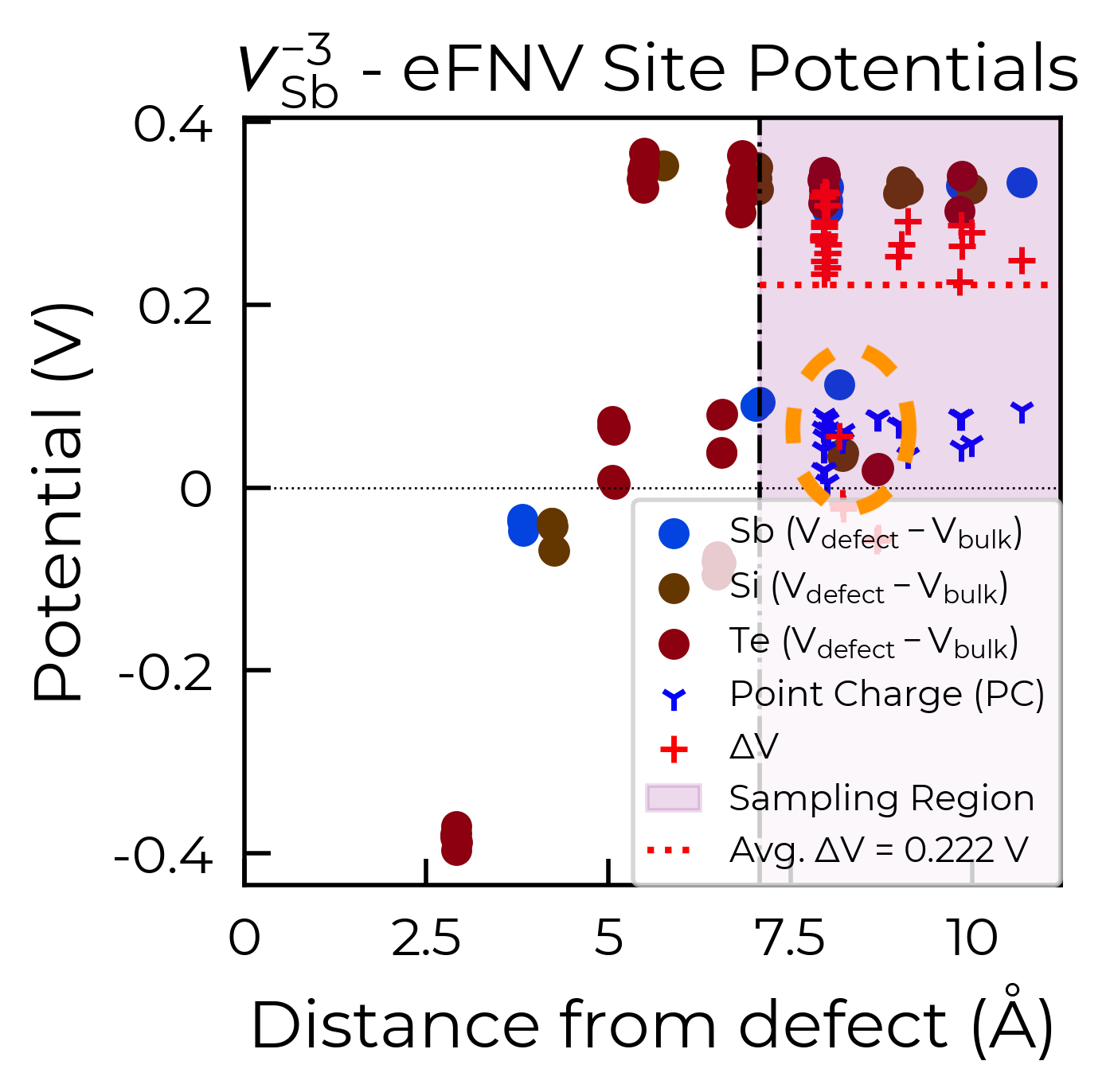
From the eFNV plot, we can see that there appears to be two distinct sets of site potentials, with one curving up from ~-0.4 V to ~0.1 V, and another mostly constant set at ~0.3 V. We can understand this by considering the structure of our defect (shown on the right), where the location of the Sb vacancy (hidden by the projection along the plane) is circled in green – we can see the displacement of the Sb atoms on either side.

Due to the layered structure, the charge and strain associated with the defect is mostly confined to the defective layer, while that of the layer away from the defect mostly experiences the typical long-range electostatic potential of the defect charge. The same behaviour can be seen for h-BN in the original eFNV paper (Figure 4d). This means that our usual default of using the Wigner-Seitz radius to determine the sampling region is not as good, as it’s including sites in the defective layer (circled in orange) which are causing the variance in the potential offset (ΔV) and thus the error in the charge correction.

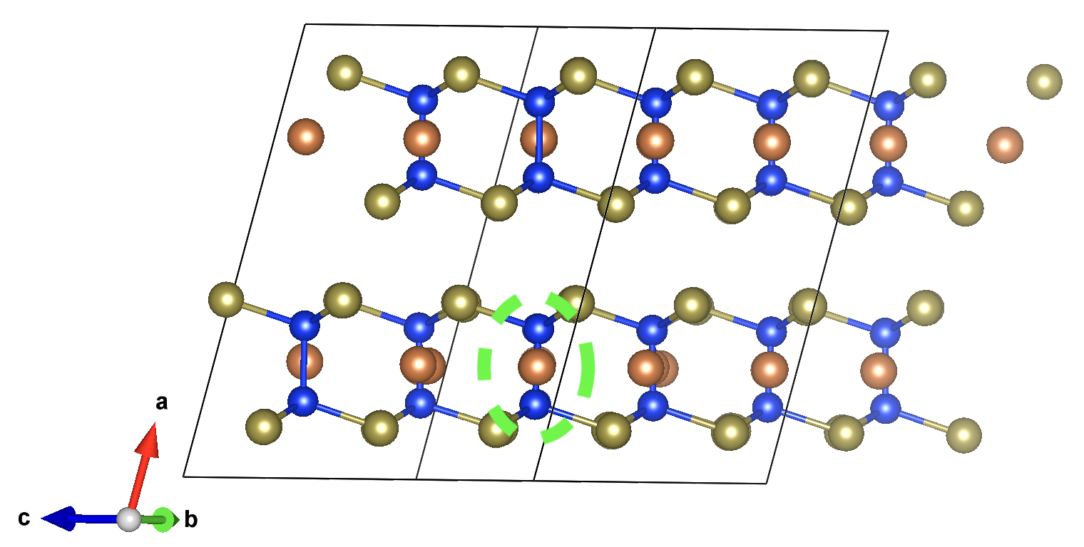
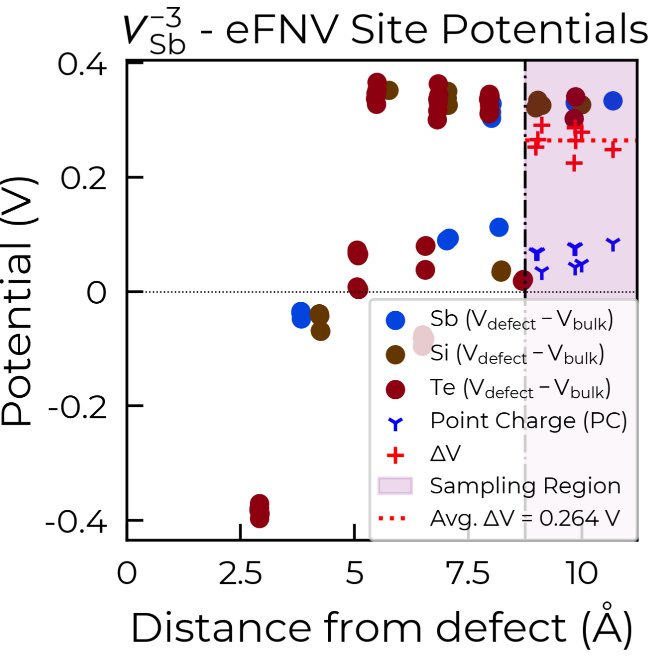
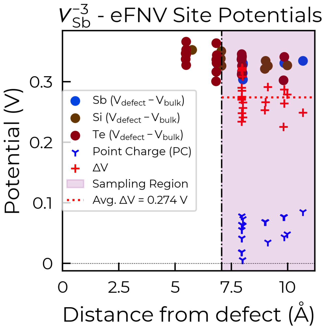
To fix this, we can use the optional defect_region_radius or excluded_indices parameters in get_kumagai_correction, to exclude those points from the sampling. For defect_region_radius, we can just set this to 8.75 Å here to avoid those sites in the defective layer. Often it may not be so simple to exclude the intra-layer sites in this way (depending on the supercell), and so alternatively we can use excluded_indices for more fine-grained control. As we can see in the structure image above, the a lattice vector is aligned along the inter-layer direction, so we can determine the intra-layer sites using the fractional coordinates of the defect site along a:

# get indices of sites within 0.2 fractional coordinates along a of the defect site
sites_in_layer = [
    i for i, site in enumerate(defect_entry.defect_supercell)
    if abs(site.frac_coords[0] - defect_entry.defect_supercell_site.frac_coords[0]) < 0.2
]
correction, fig =  dp.defect_dict["v_Sb-3"].get_kumagai_correction(
    excluded_indices=sites_in_layer, plot=True
)  # note that this updates the DefectEntry.corrections value, so the updated correction
# is used in later formation energy / concentration calculations

Below are the two resulting charge correction plots (using defect_region_radius on the left, and excluded_indices on the right):

Eigenvalue / Electronic Structure Analysis

In doped, we can use the DefectEntry.get_eigenvalue_analysis() method to analyse the orbital character and localisation of single-particle eigenstates from the underlying electronic structure calculations. For this, we employ the methodology of Kumagai et al. (through an interface with pydefect), which allows in-depth analysis of localised/deep in-gap defect states and their effects on the band edges, as well as the automated identification of shallow / perturbed host states (PHS) – see the following section for an example of this analysis. The easyunfold package for band structure unfolding can also be quite useful for extending this electronic structure analysis.

The optional argument parse_projected_eigen in DefectsParser (True by default) controls whether to load the projected eigenvalues & orbitals, which then allows DefectEntry.get_eigenvalue_analysis() to be called – returning information about the nature of the band edge and in-gap states, allowing defect states (and whether they are deep or shallow/PHS) to be automatically identified and characterised. Furthermore, a plot of the single-particle electronic eigenvalues is returned (if plot = True; default). Note that for VASP to output the necessary data for this analysis, your INCAR file needs to include LORBIT > 10 (to obtain the projected orbitals).

In the examples below (both of which are shown in the advanced analysis tutorial), we plot the single particle levels for the cadmium vacancy in CdTe (V_Cd) in each of its charge states (0, -1 and -2); calculated with spin-orbit coupling (SOC) and a 2x2x2 k-point mesh:

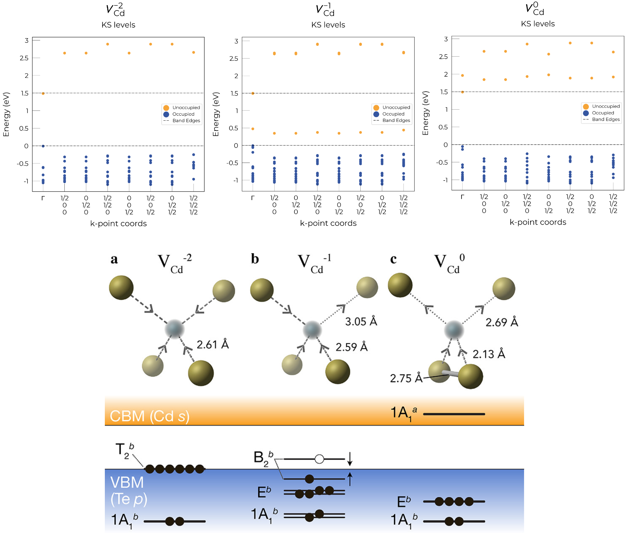
Here we can see that these plots nicely match the schematic depiction from this paper on vacancies in CdTe, where we have no in-gap states for the fully-ionised V_Cd^-2 as expected, an in-gap hole polaron state for V_Cd^-1, and an anti-bonding dimer state for V_Cd⁰ just above the CBM.

Perturbed Host States (Shallow Defects)

One of the most common reasons for performing this electronic structure analysis is to identify and analyse shallow defect states. Certain point defects form shallow (hydrogen-like) donor or acceptor states, known as perturbed host states (PHS). These states typically have wavefunctions distributed over many unit cells in real space, requiring exceptionally large supercells or dense reciprocal space sampling to properly capture their physics (see this review). This weak attraction of the electron/hole to the defect site corresponds to a relatively small donor/acceptor binding energy (i.e. energetic separation of the corresponding charge transition level to the nearby band edge), which is typically <100 meV.

Current supercell correction schemes can not accurately account for finite-size errors obtained when calculating the energies of PHS (shallow defect states) in moderate supercells, so it is recommended to denote such shallow defects as PHS and conclude only qualitatively that their transition level is located near the corresponding band edge. An example of this is given in Kikuchi et al. Chem. Mater. 2020.

Tip

Typically, the shallow defect binding energy can be reasonably well estimated using the hydrogenic model, similar to the Wannier-Mott exciton model, which predicts a binding energy given by:

\[E_b = \text{13.6 eV} \times \frac{\bar{m}}{\epsilon^2}\]

where \(\bar{m}\) is the harmonic mean (i.e. conductivity) effective mass of the relevant charge-carrier (electron/hole), \(\epsilon\) is the total dielectric constant (\(\epsilon = \epsilon_{\text{ionic}} + \epsilon_{\infty}\)) and 13.6 eV is the Rydberg constant (i.e. binding energy of an electron in a hydrogen atom).

As discussed in the section above, we employ the methodology of Kumagai et al. to analyse the orbital character and localisation of single-particle eigenstates from the underlying electronic structure calculations, which allows the automated identification of shallow states.

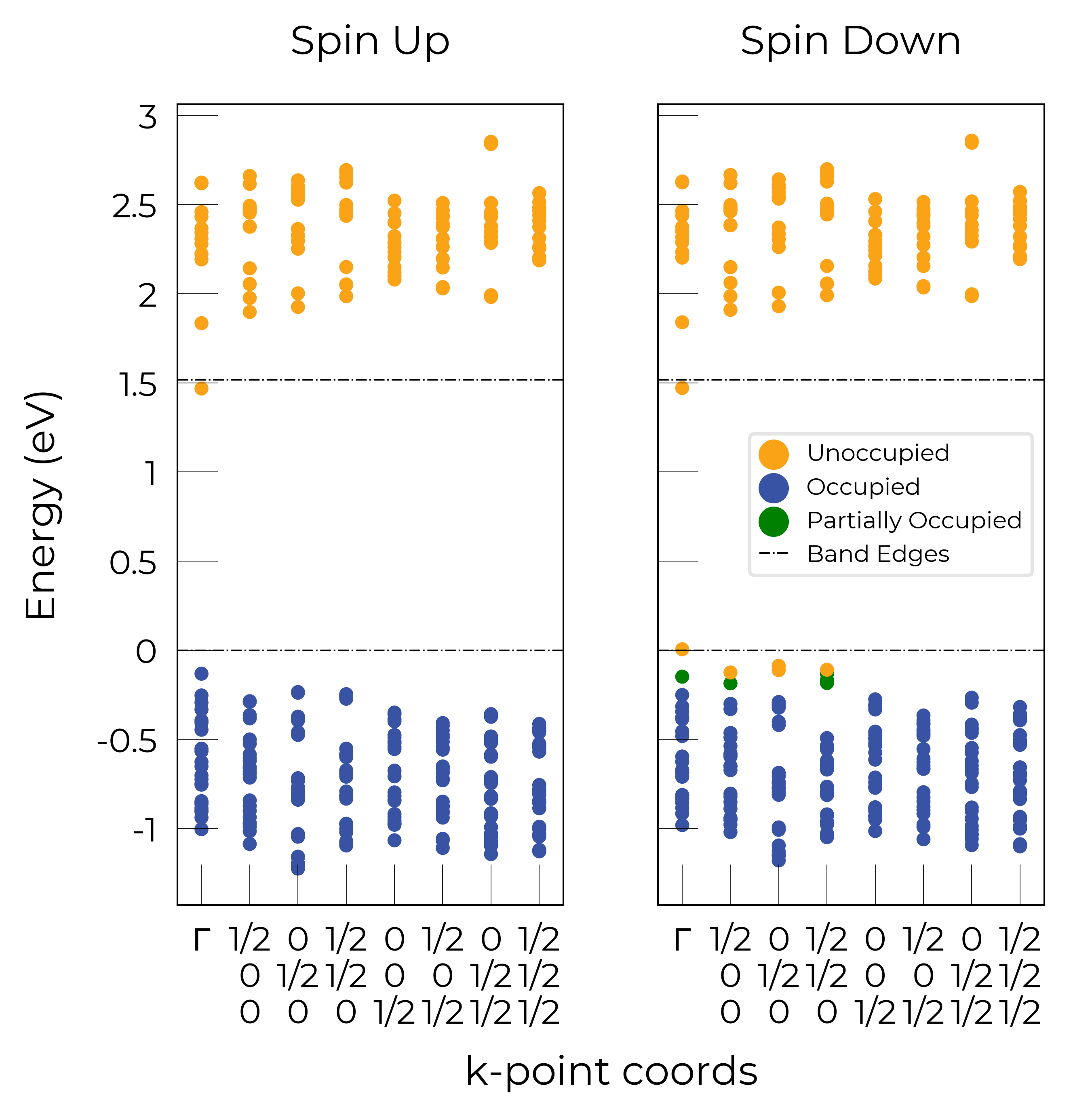
In the example below, the neutral copper vacancy in Cu₂SiSe₃ was determined to be a PHS. This was additionally confirmed by performing calculations in larger supercells and plotting the charge density. Important terms include:

1. P-ratio: The ratio of the summed projected orbital contributions of the defect & neighbouring sites to the total sum of orbital contributions from all atoms to that electronic state. A value close to 1 indicates a localised state.

2. Occupation: Occupation of the electronic state / orbital.

3. vbm has acceptor phs/cbm has donor phs: Whether a PHS has been automatically identified. Depends on how VBM-like/CBM-like the defect states are and the occupancy of the state. (X vs. 0.2) refers to the hole/electron occupancy at the band edge vs the default threshold of 0.2 for flagging as a PHS (but you should use your own judgement of course).

4. Localized Orbital(s): Information about localised defect states, if present.

Additionally, Index refers to the band/eigenvalue index in the DFT calculation, Energy is its eigenvalue energy at the given K-point coords, Orbitals lists the projected orbital contributions to that state, and OrbDiff is the normalised difference in projected orbital contributions to the VBM/CBM states between the bulk and defect supercells.

bulk = "Cu2SiSe3/bulk/vasp_std"
defect = "Cu2SiSe3/v_Cu_0/vasp_std/"
dielectric = [[8.73, 0, -0.48],[0., 7.78, 0],[-0.48, 0, 10.11]]

defect_entry = DefectParser.from_paths(defect, bulk, dielectric).defect_entry
bes, fig = defect_entry.get_eigenvalue_analysis()
print(bes)  # print information about the defect state

 -- band-edge states info
Spin-up
     Index  Energy  P-ratio  Occupation  OrbDiff  Orbitals                            K-point coords
VBM  347    3.539   0.05     1.00        0.01     Cu-d: 0.35, Se-p: 0.36              ( 0.000,  0.000,  0.000)
CBM  348    5.139   0.03     0.00        0.03     Se-s: 0.20, Se-p: 0.11, Si-s: 0.13  ( 0.000,  0.000,  0.000)
vbm has acceptor phs: False (0.000 vs. 0.2)
cbm has donor phs: False (0.000 vs. 0.2)
---
Localized Orbital(s)
Index  Energy  P-ratio  Occupation  Orbitals

Spin-down
     Index  Energy  P-ratio  Occupation  OrbDiff  Orbitals                            K-point coords
VBM  347    3.677   0.06     0.00        0.01     Cu-d: 0.34, Se-p: 0.35              ( 0.000,  0.000,  0.000)
CBM  348    5.142   0.04     0.00        0.03     Se-s: 0.20, Se-p: 0.11, Si-s: 0.13  ( 0.000,  0.000,  0.000)
vbm has acceptor phs: True (1.000 vs. 0.2)
cbm has donor phs: False (0.000 vs. 0.2)
---
Localized Orbital(s)
Index  Energy  P-ratio  Occupation  Orbitals

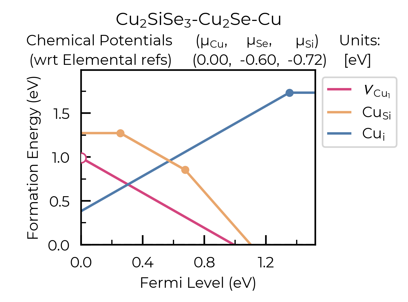
The plot of the single particle levels is shown below (left), and an example of how you might chose to represent the PHS on the transition level diagram with a clear circle is shown on the right.

Note

It is recommended to additionally manually check the real-space charge density (i.e. PARCHG) of the defect state to confirm the identification of a PHS.

Spin Polarisation

Proper accounting of spin polarisation and multiplicity is crucial for accurate defect calculations and analysis. For defect species with odd numbers of electrons (and thus being open-shell), they will adopt non-zero integer spin states, while defect species with even numbers of electrons can be either closed-shell (spin-paired) or open-shell (spin-active), depending on the defect species and its electronic structure. As such, defect calculations should typically be performed with spin polarisation allowed in all cases (i.e. with ISPIN = 2 in VASP).

Tip

If we have (nearly) converged the geometry relaxation for an even-electron defect species and there is no non-zero magnetic moments on any site (given by the magnetization output in the OUTCAR file) – and so adopting a closed-shell electronic structure, then we can set ISPIN = 1 (turning off spin polarisation) for subsequent calculations to reduce the computational cost.

The snb-mag --verbose CLI command from ShakeNBreak can be used to automatically check the magnetisation of a VASP defect calculation in this way (and is automatically used by snb-run to set ISPIN = 1 for continued ShakeNBreak relaxations of any closed-shell defect calculations, if it is being used to manage the structure-searching calculations).

❯ snb-mag -h
Usage: snb-mag [OPTIONS]

  Checks if the magnetisation (spin polarisation) values of all atoms in the
  VASP calculation are below a certain threshold, by pulling this data from
  the OUTCAR. Returns a shell exit status of 0 if magnetisation is below the
  threshold and 1 if above.

Options:
  -o, --outcar FILE      Path to OUTCAR(.gz) file
  -t, --threshold FLOAT  Atoms with absolute magnetisation below this value
                         are considered un-magnetised / non-spin-polarised.
                         The threshold for total magnetisation is 10x this
                         value.  [default: 0.01]
  -v, --verbose          Print information about the magnetisation of the
                         system.
  -h, --help             Show this message and exit.

In most cases and particularly for s/p orbital systems, odd electron defects will adopt a doublet spin state (S = 1/2, one unpaired electron), while even electron defects will tend to adopt a closed-shell singlet spin state (S = 0, no unpaired electrons), as a consequence of the Aufbau principle and Hund’s rule. This is the default logic assumed in doped (and ShakeNBreak), where the expected spin state is enforced by setting NUPDOWN (number of unpaired electrons) to 0 for even-electron and 1 for odd-electron defect species.

However, this is not always the case and often we can have open-shell triplet states for even-electron defects (with S = 1, two unpaired electrons) or quartet states for odd-electron defects (with S = 3/2, three unpaired electrons). Such cases are most common when the defect species adopts a bipolaron/multi-polaron state (e.g. for V_Cd^0* in CdTe), a molecular dimer-like state (such as O₂ species in oxides, or carbon pairs in silicon) or with orbital-degenerate/correlated defects where Hund’s rule implies open-shell solutions (such as the highly-studied NV centre in diamond or transition metal impurities in silicon). If you encounter defect states like these and/or suspect that alternative spin configurations may be possible, you should test the different possibilities by setting NUPDOWN (and possibly MAGMOM, discussed below) accordingly – ideally performing the full structure-searching calculations for these species with these settings, as the potential energy surface can differ significantly under different spin states.

Note

In general, it is best to explicitly specify the system spin state (i.e. with NUPDOWN) in DFT calculations, rather than leaving this as a free parameter, as not enforcing this constraint can often lead to erroneous and unphysical results in the form of partial orbital occupation and spins. This can occur because the DFT self-interaction error initially favours delocalisation of the unpaired electron density, and converges to this unphysical result.

As well as setting the total spin state of our supercell with NUPDOWN, another parameter that can be important in certain cases is the individual site magnetic moments, which can be initialised with the MAGMOM tag in the INCAR (see the VASPwiki page). This tag is not set by default in doped, using the VASP default initialisation of MAGMOM = NIONS*1. This tag is particularly important for magnetic materials (as discussed in the Magnetism section of the ShakeNBreak tips page), and can be useful if trying to favour a specific polaron/spin configuration (as briefly discussed at this point in the YouTube defects tutorial). This tag can be set using the user_incar_settings parameter in the doped.vasp classes, for which the python API helps streamline this process when setting MAGMOM for multiple defects.

Note

For magnetic competing phases, the spin configuration should also be appropriately set. doped will automatically set NUPDOWN according to the magnetisation output from the Materials Project calculation of the competing phase, but MAGMOM may also need to be set to induce a specific spin configuration.

Symmetry Precision (symprec)

When computing the symmetries of structures, a threshold parameter has to be set in order to distinguish structural/positional noise from distinct site differences. In doped as in spglib (and pymatgen), this can be controlled with the symprec parameter (which can be set in DefectsParser, DefectParser, all DefectThermodynamics symmetry/concentration functions, get_orientational_degeneracy(), point_symmetry_from_defect_entry() and others).

By default, doped uses a value of symprec = 0.01 for unrelaxed/bulk structures (matching the pymatgen default), and a larger symprec = 0.1 for determining the point symmetries (and thus orientational degeneracies) of relaxed defect structures to account for residual structural noise. This symprec value of 0.1 also matches that used by the Materials Project. You may want to adjust symprec for your system (e.g. if there are very slight octahedral distortions etc.).

Tip

Note that you can directly use the point_symmetry function from doped.utils.symmetry (see the docstring in the python API docs) to obtain the relaxed or unrelaxed (bulk site) point symmetries of a given defect supercell, directly from just the relaxed structures, regardless of whether these defects were generated/parsed with doped.

Serialization & Data Provenance (JSON/csv)

To aid calculation reproducibility, data provenance and easy sharing/comparison of pre- and post-processing stages of the defect workflow, doped objects have been made fully serializable, meaning they can be easily saved and (re-)loaded from compact, lightweight .json files. As demonstrated at various stages in the tutorials, this can be achieved using the dumpfn/loadfn functions from monty.serialization, or with the to_json/from_json methods provided for Defect, DefectEntry, DefectsGenerator and DefectThermodynamics objects:

# save a DefectThermodynamics object to a JSON file
defect_thermo.to_json("MgO_DefectThermodynamics.json")

# then later in a different python session or notebook, we can reload the
# DefectThermodynamics object from the JSON file, containing all the associated info
from doped.thermodynamics import DefectThermodynamics
defect_thermodynamics = DefectThermodynamics.from_json("MgO_DefectThermodynamics.json")

# alternatively, we can directly use the monty dumpfn/loadfn functions
# directly on any doped object, e.g. with our ``DefectsSet`` object
# containing all the info on the generated VASP input files:
from monty.serialization import dumpfn, loadfn
dumpfn(obj=defects_set, fn="MgO_DefectsSet.json")

# and again later reload the object from the JSON file
defects_set = loadfn("MgO_DefectsSet.json")

Note

While these JSON files tend to have relatively small file sizes anyway, we can further reduce their size by saving to / loading from gzip or bz2 compressed JSON files, by specifying .json.gz/.json.z/.json.bz2 as the file extension in the serialization functions.

In the typical defect calculation workflow with doped (exemplified in the tutorials), the following JSON files are automatically written to file:

• The DefectsGenerator object or defect_entries dictionary that is input to DefectsSet, when writing VASP input files with DefectsSet.write_files(output_path=".") – written to output_path. Additionally, for each calculation directory generated, the corresponding DefectEntry object is written to a {DefectEntry.name}.json file in the directory so that all information on the generated defect structure, charge state etc. is preserved in the calculation directory.

• The parsed defect entries dict (DefectsParser.defect_dict) when defect calculations are parsed with DefectsParser(output_path=".") – written to output_path. The JSON filename can be set with e.g. DefectsParser(json_filename="custom_name.json"), but the default is {Host Chemical Formula}_defect_dict.json.

  • Additionally, a voronoi_nodes.json file is saved to the bulk supercell calculation directory if any interstitial defects are parsed. This contains information about the Voronoi tessellation nodes in the host structure, which are used for analysing interstitial positions but can be somewhat costly to calculate – so are automatically saved to file once initially computed to reduce parsing times.

• Additionally, if following the recommended structure-searching approach with ShakeNBreak as shown in the tutorials, distortion_metadata.json files will be written to the top directory (output_path, containing distortion information about all defects) and to each defect directory (containing just the distortion information for that defect) when running Dist.write_vasp_files(output_path=".").

In most cases it is also recommended to save the DefectThermodynamics object to file once generated (using DefectThermodynamics.to_json()), to avoid having to re-parse at any later stage, however this is not done automatically.

DataFrame Outputs

Many analysis methods in doped return pandas DataFrame objects as the result, such as the get_symmetries_and_degeneracies(), get_formation_energies(), get_equilibrium_concentrations(), get_quenched_fermi_level_and_concentrations, get_dopability_limits(), get_doping_windows() and get_transition_levels() methods for DefectThermodynamics objects, and the formation_energy_df attribute and calculate_chempots() method for CompetingPhasesAnalyzer. As mentioned in the tutorials, these DataFrame objects can be output to csv (or json, xlsx etc., see the pandas API docs here) using the to_csv/to_json methods:

# save the formation energies DataFrame to a csv file
defect_thermo.get_formation_energies().to_csv("MgO_formation_energies.csv")

These csv files can easily be used as data tables when writing up results, by directly importing to Microsoft Word or converting to LaTeX format using Tables Generator. CompetingPhasesAnalyzer can also be reinitialised from a saved csv formation energies file with the from_csv() method.

Note

Have any tips for users from using doped? Please share it with the developers and we’ll add them here!