Generating defects with doped
If you are new to computational modelling of defects, it is highly recommended that you watch the defect calculations tutorial (YouTube, B站) and see the docs Literature section. This gives a brief overview of much of the theory and rationale behind our typical defect calculation workflow.
In this tutorial we show how to generate defects and VASP input files with doped, and also perform
the recommended ShakeNBreak structure-searching step at the beginning of the defect workflow.
The table of contents of this tutorial is shown in the left-hand sidebar, and you can click on any of the
links to jump to that section.
Tip
You can run this notebook interactively through Google Colab or Binder – just click the links! (Then uncomment the !pip install... cell).
# # If running on Colab; uncomment to install doped, clone the repo to download the example data and cd in to examples folder:
# !pip install doped
# !git clone https://github.com/SMTG-Bham/doped
# %cd doped/examples
# # Note that when running on Colab, POTCAR file generation will not be possible as this requires the VASP POTCAR directory
# # to be setup with pymatgen (see https://doped.readthedocs.io/en/latest/Installation.html), but all other parts of this
# # notebook can be run directly
Defect Generation
from pymatgen.core.structure import Structure
from doped.generation import DefectsGenerator
# generate defects in our relaxed bulk (host) structure:
defect_gen = DefectsGenerator("CdTe/relaxed_primitive_POSCAR")  # can also provide as Structure object
Generating DefectEntry objects: 100.0%|██████████| [00:02, 37.63it/s]
Vacancies    Guessed Charges    Conv. Cell Coords    Wyckoff
-----------  -----------------  -------------------  ---------
v_Cd         [+1,0,-1,-2]       [0.000,0.000,0.000]  4a
v_Te         [+2,+1,0,-1]       [0.250,0.250,0.250]  4c

Substitutions    Guessed Charges        Conv. Cell Coords    Wyckoff
---------------  ---------------------  -------------------  ---------
Cd_Te            [+4,+3,+2,+1,0]        [0.250,0.250,0.250]  4c
Te_Cd            [+2,+1,0,-1,-2,-3,-4]  [0.000,0.000,0.000]  4a

Interstitials    Guessed Charges        Conv. Cell Coords    Wyckoff
---------------  ---------------------  -------------------  ---------
Cd_i_C3v         [+2,+1,0]              [0.625,0.625,0.625]  16e
Cd_i_Td_Cd2.83   [+2,+1,0]              [0.750,0.750,0.750]  4d
Cd_i_Td_Te2.83   [+2,+1,0]              [0.500,0.500,0.500]  4b
Te_i_C3v         [+4,+3,+2,+1,0,-1,-2]  [0.625,0.625,0.625]  16e
Te_i_Td_Cd2.83   [+4,+3,+2,+1,0,-1,-2]  [0.750,0.750,0.750]  4d
Te_i_Td_Te2.83   [+4,+3,+2,+1,0,-1,-2]  [0.500,0.500,0.500]  4b

The number in the Wyckoff label is the site multiplicity/degeneracy of that defect in the conventional ('conv.') unit cell, which comprises 4 formula unit(s) of CdTe.
The DefectsGenerator class is used to generate defects with doped.
It has been set up to adopt reasonable defaults, such as supercell generation (tries to find the smallest possible supercell which is at least 10 Å in each direction; a typical threshold for minimising finite-size effects) and defect charge state guessing, but these are fully customisable using the class options shown in the docstring below and illustrated in the Custom Supercell Generation section of the advanced analysis tutorial.
By default, defects are placed at the closest possible symmetry-equivalent site to the midpoint of the supercell, to aid visualisation e.g. in VESTA.
Important
As always with defect studies, you should carefully consider whether the default settings are appropriate for your system, and if not, you should customise them accordingly.
Some typical reasons for customising the default settings include:
Guessed Charges: The
dopedcharge-state guessing algorithm has been developed to try balance efficiency (avoiding unnecessary calculations) and completeness (avoiding missing out on important defect species). However often defects behave in ways that we mightn’t expect at first (part of what makes them interesting!) and so no algorithm is able to predict exactly which charge states will/won’t be stable for your system. So, you should consider if your system is likely to have any unusual charge states (e.g. common in systems with low-symmetry (e.g. Sb₂Se₃), defect reconstructions (e.g. Sb₂S₃ & Al₂O₃ and/or amphoteric species (e.g. CdTe)) and if so, you should update the charge state ranges of your defects accordingly (example shown below).Supercell Generation: You may want to adjust the default supercell generation constraints (using
supercell_gen_kwargs– see docstrings and Custom Supercell Generation), particularly for hard materials or those with low dielectric constants (where finite-size effects such as strain & image charge interactions are likely to be more significant) or highly-anisotropic (e.g. 2D/layered) materials (where dielectric-weighted supercell generation may be most efficient).Target Supercell: You may want to use a specific supercell for your calculations, perhaps to reproduce or build on calculations from a previous study with a specific supercell, which can be easily achieved by providing the desired supercell and setting
DefectsGenerator(..., generate_supercell=False).
# run this to see the function documentation:
DefectsGenerator?
Information about the generated defects and supercell is accessible using the DefectsGenerator
attributes, like defect_entries, bulk_supercell, defects etc.
Note
Note:
The algorithm for determining defect entry names is to use the pymatgen defect
name (e.g. v_Cd, Cd_Te etc.) for vacancies/antisites/substitutions, unless
there are multiple inequivalent sites for the defect, in which case the point
group of the defect site is appended (e.g. v_Cd_Td, Cd_Te_Td etc.), and if
this is still not unique, then element identity and distance to the nearest
neighbour of the defect site is appended (e.g. v_Cd_Td_Te2.83, Cd_Te_Td_Cd2.83
etc.). For interstitials, the same naming scheme is used, but the point group
is always appended to the pymatgen defect name.
Remember that these are the point groups of the initial, unrelaxed defect structures! Which are likely to change during geometry relaxation (see e.g. 10.1039/D2FD00043A, 10.1038/s41578-025-00879-y, or 10.1039/D3CS00432E for a discussion on this and the corresponding effects on configurational degeneracies).
# show the generated defect entries:
defect_gen.defect_entries.keys()
dict_keys(['v_Cd_+1', 'v_Cd_0', 'v_Cd_-1', 'v_Cd_-2', 'v_Te_+2', 'v_Te_+1', 'v_Te_0', 'v_Te_-1', 'Cd_Te_+4', 'Cd_Te_+3', 'Cd_Te_+2', 'Cd_Te_+1', 'Cd_Te_0', 'Te_Cd_+2', 'Te_Cd_+1', 'Te_Cd_0', 'Te_Cd_-1', 'Te_Cd_-2', 'Te_Cd_-3', 'Te_Cd_-4', 'Cd_i_C3v_+2', 'Cd_i_C3v_+1', 'Cd_i_C3v_0', 'Cd_i_Td_Cd2.83_+2', 'Cd_i_Td_Cd2.83_+1', 'Cd_i_Td_Cd2.83_0', 'Cd_i_Td_Te2.83_+2', 'Cd_i_Td_Te2.83_+1', 'Cd_i_Td_Te2.83_0', 'Te_i_C3v_+4', 'Te_i_C3v_+3', 'Te_i_C3v_+2', 'Te_i_C3v_+1', 'Te_i_C3v_0', 'Te_i_C3v_-1', 'Te_i_C3v_-2', 'Te_i_Td_Cd2.83_+4', 'Te_i_Td_Cd2.83_+3', 'Te_i_Td_Cd2.83_+2', 'Te_i_Td_Cd2.83_+1', 'Te_i_Td_Cd2.83_0', 'Te_i_Td_Cd2.83_-1', 'Te_i_Td_Cd2.83_-2', 'Te_i_Td_Te2.83_+4', 'Te_i_Td_Te2.83_+3', 'Te_i_Td_Te2.83_+2', 'Te_i_Td_Te2.83_+1', 'Te_i_Td_Te2.83_0', 'Te_i_Td_Te2.83_-1', 'Te_i_Td_Te2.83_-2'])
If we wanted to manually add some extra charge states (e.g. some negative charge states for Cd_Te), we
can do so using the add_charge_states method:
# Add some extra charge states for Cd_Te antisites
defect_gen.add_charge_states(defect_entry_name="Cd_Te", charge_states=[-2, -1])
# check our generated defect entries:
defect_gen
DefectsGenerator for input composition CdTe, space group F-43m with 52 defect entries created.
---------------------------------------------------------
Vacancies    Guessed Charges    Conv. Cell Coords    Wyckoff
-----------  -----------------  -------------------  ---------
v_Cd         [+1,0,-1,-2]       [0.000,0.000,0.000]  4a
v_Te         [+2,+1,0,-1]       [0.250,0.250,0.250]  4c

Substitutions    Guessed Charges        Conv. Cell Coords    Wyckoff
---------------  ---------------------  -------------------  ---------
Cd_Te            [+4,+3,+2,+1,0,-1,-2]  [0.250,0.250,0.250]  4c
Te_Cd            [+2,+1,0,-1,-2,-3,-4]  [0.000,0.000,0.000]  4a

Interstitials    Guessed Charges        Conv. Cell Coords    Wyckoff
---------------  ---------------------  -------------------  ---------
Cd_i_C3v         [+2,+1,0]              [0.625,0.625,0.625]  16e
Cd_i_Td_Cd2.83   [+2,+1,0]              [0.750,0.750,0.750]  4d
Cd_i_Td_Te2.83   [+2,+1,0]              [0.500,0.500,0.500]  4b
Te_i_C3v         [+4,+3,+2,+1,0,-1,-2]  [0.625,0.625,0.625]  16e
Te_i_Td_Cd2.83   [+4,+3,+2,+1,0,-1,-2]  [0.750,0.750,0.750]  4d
Te_i_Td_Te2.83   [+4,+3,+2,+1,0,-1,-2]  [0.500,0.500,0.500]  4b

The number in the Wyckoff label is the site multiplicity/degeneracy of that defect in the conventional ('conv.') unit cell, which comprises 4 formula unit(s) of CdTe.
We see that -2 and -1 charge states have now been added for our Cd-on-Te antisite substitution.
Again, the help documentation for this function can be viewed with by adding a question mark to the function/method name:
# run this to see the function documentation:
defect_gen.add_charge_states?
# likewise we can remove charge states with:
defect_gen.remove_charge_states(defect_entry_name="v_Cd", charge_states=[+1])
defect_gen
DefectsGenerator for input composition CdTe, space group F-43m with 51 defect entries created.
---------------------------------------------------------
Vacancies    Guessed Charges    Conv. Cell Coords    Wyckoff
-----------  -----------------  -------------------  ---------
v_Cd         [0,-1,-2]          [0.000,0.000,0.000]  4a
v_Te         [+2,+1,0,-1]       [0.250,0.250,0.250]  4c

Substitutions    Guessed Charges        Conv. Cell Coords    Wyckoff
---------------  ---------------------  -------------------  ---------
Cd_Te            [+4,+3,+2,+1,0,-1,-2]  [0.250,0.250,0.250]  4c
Te_Cd            [+2,+1,0,-1,-2,-3,-4]  [0.000,0.000,0.000]  4a

Interstitials    Guessed Charges        Conv. Cell Coords    Wyckoff
---------------  ---------------------  -------------------  ---------
Cd_i_C3v         [+2,+1,0]              [0.625,0.625,0.625]  16e
Cd_i_Td_Cd2.83   [+2,+1,0]              [0.750,0.750,0.750]  4d
Cd_i_Td_Te2.83   [+2,+1,0]              [0.500,0.500,0.500]  4b
Te_i_C3v         [+4,+3,+2,+1,0,-1,-2]  [0.625,0.625,0.625]  16e
Te_i_Td_Cd2.83   [+4,+3,+2,+1,0,-1,-2]  [0.750,0.750,0.750]  4d
Te_i_Td_Te2.83   [+4,+3,+2,+1,0,-1,-2]  [0.500,0.500,0.500]  4b

The number in the Wyckoff label is the site multiplicity/degeneracy of that defect in the conventional ('conv.') unit cell, which comprises 4 formula unit(s) of CdTe.
If we want to generate defects with extrinsic elements, to investigate doping or potential impurities in
the material, we can do so using the extrinsic option. This can be either a string of a single
impurity element to consider, a list of multiple possible extrinsic species, or a dictionary in the
form {host_element: extrinsic_element} if we only want to consider specific substitutions
host/impurity substitutions.
For example, to investigate Cu, Se and Na doping in CdTe, we can do:
relaxed_primitive_CdTe = Structure.from_file("CdTe/relaxed_primitive_POSCAR")
extrinsic_defect_gen = DefectsGenerator(relaxed_primitive_CdTe, extrinsic=["Cu", "Se", "Na"])
Generating DefectEntry objects: 100.0%|██████████| [00:02, 40.28it/s]
Vacancies    Guessed Charges    Conv. Cell Coords    Wyckoff
-----------  -----------------  -------------------  ---------
v_Cd         [+1,0,-1,-2]       [0.000,0.000,0.000]  4a
v_Te         [+2,+1,0,-1]       [0.250,0.250,0.250]  4c

Substitutions    Guessed Charges        Conv. Cell Coords    Wyckoff
---------------  ---------------------  -------------------  ---------
Cd_Te            [+4,+3,+2,+1,0]        [0.250,0.250,0.250]  4c
Te_Cd            [+2,+1,0,-1,-2,-3,-4]  [0.000,0.000,0.000]  4a
Na_Cd            [0,-1]                 [0.000,0.000,0.000]  4a
Na_Te            [+3,+2,+1,0]           [0.250,0.250,0.250]  4c
Cu_Cd            [+1,0,-1]              [0.000,0.000,0.000]  4a
Cu_Te            [+4,+3,+2,+1,0]        [0.250,0.250,0.250]  4c
Se_Cd            [+2,+1,0,-1,-2,-3,-4]  [0.000,0.000,0.000]  4a
Se_Te            [+1,0]                 [0.250,0.250,0.250]  4c

Interstitials    Guessed Charges        Conv. Cell Coords    Wyckoff
---------------  ---------------------  -------------------  ---------
Cd_i_C3v         [+2,+1,0]              [0.625,0.625,0.625]  16e
Cd_i_Td_Cd2.83   [+2,+1,0]              [0.750,0.750,0.750]  4d
Cd_i_Td_Te2.83   [+2,+1,0]              [0.500,0.500,0.500]  4b
Te_i_C3v         [+4,+3,+2,+1,0,-1,-2]  [0.625,0.625,0.625]  16e
Te_i_Td_Cd2.83   [+4,+3,+2,+1,0,-1,-2]  [0.750,0.750,0.750]  4d
Te_i_Td_Te2.83   [+4,+3,+2,+1,0,-1,-2]  [0.500,0.500,0.500]  4b
Na_i_C3v         [+1,0]                 [0.625,0.625,0.625]  16e
Na_i_Td_Cd2.83   [+1,0]                 [0.750,0.750,0.750]  4d
Na_i_Td_Te2.83   [+1,0]                 [0.500,0.500,0.500]  4b
Cu_i_C3v         [+2,+1,0]              [0.625,0.625,0.625]  16e
Cu_i_Td_Cd2.83   [+2,+1,0]              [0.750,0.750,0.750]  4d
Cu_i_Td_Te2.83   [+2,+1,0]              [0.500,0.500,0.500]  4b
Se_i_C3v         [0,-1,-2]              [0.625,0.625,0.625]  16e
Se_i_Td_Cd2.83   [0,-1,-2]              [0.750,0.750,0.750]  4d
Se_i_Td_Te2.83   [0,-1,-2]              [0.500,0.500,0.500]  4b

The number in the Wyckoff label is the site multiplicity/degeneracy of that defect in the conventional ('conv.') unit cell, which comprises 4 formula unit(s) of CdTe.
Tip
If we want to save our generated defects to a file, to then use later without having to rerun the
above generation functions, or use in a different notebook, or share with another user, we can do so
using the to_json and from_json methods for DefectsGenerator.
Determining the ground-state defect structures
At this point, it’s recommended that you use the ShakeNBreak approach to quickly identify the groundstate structures of your defects (or any alternative global optimisation method), before continuing on with the formation energy calculation workflow below. As detailed in the theory paper, skipping this step can result in drastically incorrect formation energies, transition levels, carrier capture (basically any property associated with defects). This approach is followed below, with a more in-depth explanation and tutorial given on the ShakeNBreak website.
Tip
For low-symmetry materials with many interstitial sites, we recommend screening out high-energy sites first, before performing full ShakeNBreak structure-searching for these. The recommended approach for this is detailed on the docs tips page.
Note
If for some reason you are not doing the recommended ShakeNBreak ground-state structure search for
your defects, you can skip ahead to the ‘Prepare VASP relaxation calculation files’ section below,
and follow the instructions listed in the Note there.
While the Python API approach described below is the recommended approach for using ShakeNBreak
(offering more control and ability to analyses structures), it can also be run from the command line, with more info found at the CLI docs section and a summary GIF in the CLI section of the Welcome page.
To generate our distorted defect structures with ShakeNBreak (SnB), we can directly input our
DefectsGenerator object to the SnB Distortions class:
from shakenbreak.input import Distortions
Dist = Distortions(  # Initialise the Distortions class with our generated CdTe defects
    defect_entries = defect_gen,
    #oxidation_states=oxidation_states,  # optionally explicitly specify oxidation states
)  # Distortions can also be initialised from a list of DefectEntry objects or Structure objects
Oxidation states were not explicitly set, thus have been guessed as {'Cd': 2.0, 'Te': -2.0}. If this is unreasonable you should manually set oxidation_states
Important
As with the doped functions, ShakeNBreak has been built and optimised to adopt reasonable
defaults that work well for most host materials, however there is again a lot of customisation and
control available, and you should carefully consider the appropriate settings and choices for your system.
The ShakeNBreak workflow is shown in more detail in the
SnB Python API tutorial on the
SnB docs, and here we just show a brief example of the main steps.
Generating VASP input files for the trial distorted structures
defects_dict, distortion_metadata = Dist.write_vasp_files() # set ``verbose=True`` for more info
Applying ShakeNBreak... Will apply the following bond distortions: ['-0.6', '-0.5', '-0.4', '-0.3', '-0.2', '-0.1', '0.0', '0.1', '0.2', '0.3', '0.4', '0.5', '0.6', 'Dimer (for vacancies)']. Then, will rattle with a std dev of 0.28 Å
Generating distorted defect structures...0.0%| | [00:00, ?it/s]
Defect: v_Cd
Number of missing electrons in neutral state: 2

Defect v_Cd in charge state: 0. Number of distorted neighbours: 2

Defect v_Cd in charge state: -1. Number of distorted neighbours: 1

Defect v_Cd in charge state: -2. Number of distorted neighbours: 0
Generating distorted defect structures...10.0%|█ | [00:00, 2.56it/s]
Defect: v_Te
Number of extra electrons in neutral state: 2

Defect v_Te in charge state: +2. Number of distorted neighbours: 0

Defect v_Te in charge state: +1. Number of distorted neighbours: 1

Defect v_Te in charge state: 0. Number of distorted neighbours: 2

Defect v_Te in charge state: -1. Number of distorted neighbours: 3
Generating distorted defect structures...20.0%|██ | [00:00, 2.08it/s]
Defect: Cd_Te
Number of extra electrons in neutral state: 4

Defect Cd_Te in charge state: +4. Number of distorted neighbours: 0

Defect Cd_Te in charge state: +3. Number of distorted neighbours: 1

Defect Cd_Te in charge state: +2. Number of distorted neighbours: 2

Defect Cd_Te in charge state: +1. Number of distorted neighbours: 3

Defect Cd_Te in charge state: 0. Number of distorted neighbours: 4

Defect Cd_Te in charge state: -1. Number of distorted neighbours: 3

Defect Cd_Te in charge state: -2. Number of distorted neighbours: 2
Generating distorted defect structures...30.0%|███ | [00:01, 1.46it/s]
Defect: Te_Cd
Number of missing electrons in neutral state: 4

Defect Te_Cd in charge state: +2. Number of distorted neighbours: 2

Defect Te_Cd in charge state: +1. Number of distorted neighbours: 3

Defect Te_Cd in charge state: 0. Number of distorted neighbours: 4

Defect Te_Cd in charge state: -1. Number of distorted neighbours: 3

Defect Te_Cd in charge state: -2. Number of distorted neighbours: 2

Defect Te_Cd in charge state: -3. Number of distorted neighbours: 1
Generating distorted defect structures...40.0%|████ | [00:02, 1.27it/s]
Defect Te_Cd in charge state: -4. Number of distorted neighbours: 0

Defect: Cd_i_C3v
Number of extra electrons in neutral state: 2

Defect Cd_i_C3v in charge state: +2. Number of distorted neighbours: 0

Defect Cd_i_C3v in charge state: +1. Number of distorted neighbours: 1

Defect Cd_i_C3v in charge state: 0. Number of distorted neighbours: 2
Generating distorted defect structures...50.0%|█████ | [00:03, 1.51it/s]
Defect: Cd_i_Td_Cd2.83
Number of extra electrons in neutral state: 2

Defect Cd_i_Td_Cd2.83 in charge state: +2. Number of distorted neighbours: 0

Defect Cd_i_Td_Cd2.83 in charge state: +1. Number of distorted neighbours: 1

Defect Cd_i_Td_Cd2.83 in charge state: 0. Number of distorted neighbours: 2
Generating distorted defect structures...60.0%|██████ | [00:04, 1.30it/s]
Defect: Cd_i_Td_Te2.83
Number of extra electrons in neutral state: 2

Defect Cd_i_Td_Te2.83 in charge state: +2. Number of distorted neighbours: 0

Defect Cd_i_Td_Te2.83 in charge state: +1. Number of distorted neighbours: 1

Defect Cd_i_Td_Te2.83 in charge state: 0. Number of distorted neighbours: 2
Generating distorted defect structures...70.0%|███████ | [00:05, 1.23it/s]
Defect: Te_i_C3v
Number of missing electrons in neutral state: 2

Defect Te_i_C3v in charge state: +4. Number of distorted neighbours: 2

Defect Te_i_C3v in charge state: +3. Number of distorted neighbours: 3

Defect Te_i_C3v in charge state: +2. Number of distorted neighbours: 4

Defect Te_i_C3v in charge state: +1. Number of distorted neighbours: 3

Defect Te_i_C3v in charge state: 0. Number of distorted neighbours: 2

Defect Te_i_C3v in charge state: -1. Number of distorted neighbours: 1
Generating distorted defect structures...80.0%|████████ | [00:06, 1.18it/s]
Defect Te_i_C3v in charge state: -2. Number of distorted neighbours: 0

Defect: Te_i_Td_Cd2.83
Number of missing electrons in neutral state: 2

Defect Te_i_Td_Cd2.83 in charge state: +4. Number of distorted neighbours: 2

Defect Te_i_Td_Cd2.83 in charge state: +3. Number of distorted neighbours: 3

Defect Te_i_Td_Cd2.83 in charge state: +2. Number of distorted neighbours: 4

Defect Te_i_Td_Cd2.83 in charge state: +1. Number of distorted neighbours: 3

Defect Te_i_Td_Cd2.83 in charge state: 0. Number of distorted neighbours: 2

Defect Te_i_Td_Cd2.83 in charge state: -1. Number of distorted neighbours: 1
Generating distorted defect structures...90.0%|█████████ | [00:06, 1.14it/s]
Defect Te_i_Td_Cd2.83 in charge state: -2. Number of distorted neighbours: 0

Defect: Te_i_Td_Te2.83
Number of missing electrons in neutral state: 2

Defect Te_i_Td_Te2.83 in charge state: +4. Number of distorted neighbours: 2

Defect Te_i_Td_Te2.83 in charge state: +3. Number of distorted neighbours: 3

Defect Te_i_Td_Te2.83 in charge state: +2. Number of distorted neighbours: 4

Defect Te_i_Td_Te2.83 in charge state: +1. Number of distorted neighbours: 3

Defect Te_i_Td_Te2.83 in charge state: 0. Number of distorted neighbours: 2

Defect Te_i_Td_Te2.83 in charge state: -1. Number of distorted neighbours: 1
Generating distorted defect structures...100.0%|██████████| [00:07, 1.26it/s]
Defect Te_i_Td_Te2.83 in charge state: -2. Number of distorted neighbours: 0
input.py:395: UserWarning: The previously-generated defect distortions folder v_Cd_0 in examples has the same Unperturbed defect structure as the current defect species: v_Cd_0. ShakeNBreak files in v_Cd_0 will be overwritten.
input.py:395: UserWarning: The previously-generated defect distortions folder v_Cd_-1 in examples has the same Unperturbed defect structure as the current defect species: v_Cd_-1. ShakeNBreak files in v_Cd_-1 will be overwritten.
input.py:395: UserWarning: The previously-generated defect distortions folder v_Cd_-2 in examples has the same Unperturbed defect structure as the current defect species: v_Cd_-2. ShakeNBreak files in v_Cd_-2 will be overwritten.
Our distorted structures and VASP input files have now been generated in the folders with names matching
the doped naming scheme:
!cat v_Cd_-1/Bond_Distortion_-10.0%/INCAR
# MAY WANT TO CHANGE NCORE, KPAR, AEXX, ENCUT, IBRION, LREAL, NUPDOWN, ISPIN, MAGMOM = Typical variable parameters
# SHAKENBREAK INCAR WITH COARSE SETTINGS TO MAXIMISE SPEED WITH SUFFICIENT ACCURACY FOR QUALITATIVE STRUCTURE SEARCHING =
AEXX = 0.25
ALGO = Normal  # change to all if zhegv, fexcp/f or zbrent errors encountered (done automatically by snb-run)
EDIFF = 1e-05
EDIFFG = -0.01
ENCUT = 300.0
GGA = Pe
HFSCREEN = 0.208
IBRION = 2
ICHARG = 1
ICORELEVEL = 0  # needed if using the kumagai-oba (efnv) anisotropic charge correction scheme
ISIF = 2
ISMEAR = 0
ISPIN = 2
ISYM = 0  # symmetry breaking extremely likely for defects
LASPH = True
LCHARG = False
LHFCALC = True
LMAXMIX = 4
LORBIT = 11
LREAL = Auto
LVHAR = True
LWAVE = False
NCORE = 16
NEDOS = 3000
NELECT = 475.0
NELM = 40
NSW = 300
NUPDOWN = 1.0
PREC = Accurate
PRECFOCK = Fast
ROPT = 1e-3 1e-3
SIGMA = 0.05
Send to HPCs and run relaxations
Can use the snb-run CLI function to quickly run calculations; see the Submitting the geometry
optimisations section of the SnB CLI tutorial for this.
For demonstration purposes in this example notebook, we’ll use some (fake) example data:
(Don’t do this if you’re actually running the calculations and have downloaded the data as instructed above)
Note
If you want to run the below functions interactively in python, you need to clone the ShakeNBreak GitHub repository and pip install the package from there (in order for the example data to be downloaded), which can be done with:
git clone https://github.com/SMTG-Bham/ShakeNBreak
cd ShakeNBreak && pip install .
import shakenbreak
from pathlib import Path

def get_repo_root(package, target_repo_name="ShakeNBreak"):
    path = Path(package.__file__).resolve()
    for parent in path.parents:
        if parent.name == target_repo_name:
            return parent
    raise FileNotFoundError(f"Repository root named '{target_repo_name}' not found.")

snb_path = get_repo_root(shakenbreak)

!rm -r v_Te* Te_* Cd_* v_Cd_*/Dimer # remove other defect folders for example case here
!cp -r {snb_path}/tests/data/example_results/v_Cd* .
!cp {snb_path}/tests/data/vasp/CdTe/distortion_metadata.json .
Plot energies vs distortion
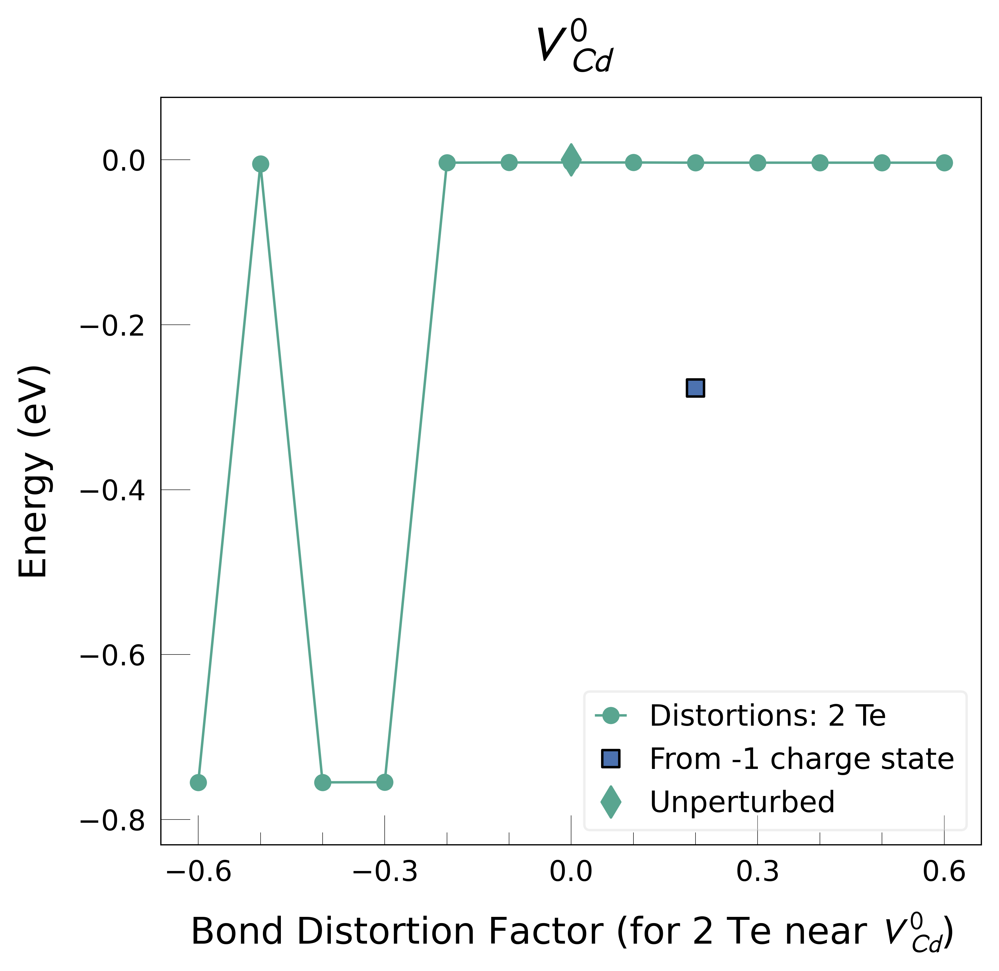
To see if SnB found any energy-lowering distortions, we can plot the results using the functions in shakenbreak.plotting. Here we show the results for cadmium vacancies only as an example:
from shakenbreak import energy_lowering_distortions, plotting
defect_charges_dict = energy_lowering_distortions.read_defects_directories()
low_energy_defects = energy_lowering_distortions.get_energy_lowering_distortions(defect_charges_dict)
v_Cd
v_Cd_0: Energy difference between minimum, found with -0.6 bond distortion, and unperturbed: -0.76 eV.
Energy lowering distortion found for v_Cd with charge 0. Adding to low_energy_defects dictionary.
v_Cd_-1: Energy difference between minimum, found with 0.2 bond distortion, and unperturbed: -0.90 eV.
New (according to structure matching) low-energy distorted structure found for v_Cd_-1, adding to low_energy_defects['v_Cd'] list.
No energy lowering distortion with energy difference greater than min_e_diff = 0.05 eV found for v_Cd with charge -2.

Comparing and pruning defect structures across charge states...
These functions give us some info about whether any energy-lowering defect distortions were identified, and we can see the results clearer by plotting:
figs = plotting.plot_all_defects(defect_charges_dict, add_colorbar=True)
For these example results, we find energy lowering distortions for VCd0 and VCd-1. We should re-test these distorted structures for the VCd charge states where these distortions were not found, in case they also give lower energies.
The get_energy_lowering_distortions() function above automatically performs structure comparisons to determine which distortions should be tested in other charge states of the same defect, and which have already been found (see docstring for more details).
# generates the new distorted structures and VASP inputs, to do our quick 2nd round of structure testing:
energy_lowering_distortions.write_retest_inputs(low_energy_defects)
Writing low-energy distorted structure to ./v_Cd_-1/Bond_Distortion_-60.0%_from_0
Writing low-energy distorted structure to ./v_Cd_-2/Bond_Distortion_-60.0%_from_0
Writing low-energy distorted structure to ./v_Cd_0/Bond_Distortion_20.0%_from_-1
Writing low-energy distorted structure to ./v_Cd_-2/Bond_Distortion_20.0%_from_-1
Again we run the calculations on the HPCs, then parse and plot the results either using the SnB CLI
functions, or through the python API as exemplified here.
# fake example data!
example_results_path = f"{snb_path}/tests/data/example_results"

!cp {example_results_path}/v_Cd_0/v_Cd_0_additional_distortions.yaml ./v_Cd_0/v_Cd_0.yaml
!cp {example_results_path}/v_Cd_-1/v_Cd_-1_additional_distortions.yaml ./v_Cd_-1/v_Cd_-1.yaml
!cp {example_results_path}/v_Cd_-2/v_Cd_-2_additional_distortions.yaml ./v_Cd_-2/v_Cd_-2.yaml
!cp {example_results_path}/v_Cd_0/Bond_Distortion_-60.0%/CONTCAR ./v_Cd_-1/Bond_Distortion_-60.0%_from_0/
!cp {example_results_path}/v_Cd_0/Bond_Distortion_-60.0%/CONTCAR ./v_Cd_-2/Bond_Distortion_-60.0%_from_0/
!cp {example_results_path}/v_Cd_-1/Unperturbed/CONTCAR ./v_Cd_-2/Bond_Distortion_20.0%_from_-1/
!cp {example_results_path}/v_Cd_-1/Unperturbed/CONTCAR ./v_Cd_0/Bond_Distortion_20.0%_from_-1/
# re-parse with the same `get_energy_lowering_distortions()` function from before:
low_energy_defects = energy_lowering_distortions.get_energy_lowering_distortions(defect_charges_dict)
v_Cd
v_Cd_0: Energy difference between minimum, found with -0.6 bond distortion, and unperturbed: -0.76 eV.
Energy lowering distortion found for v_Cd with charge 0. Adding to low_energy_defects dictionary.
v_Cd_-1: Energy difference between minimum, found with -60.0%_from_0 bond distortion, and unperturbed: -1.20 eV.
Low-energy distorted structure for v_Cd_-1 already found with charge states ['0'], storing together.
v_Cd_-2: Energy difference between minimum, found with 20.0%_from_-1 bond distortion, and unperturbed: -1.90 eV.
New (according to structure matching) low-energy distorted structure found for v_Cd_-2, adding to low_energy_defects['v_Cd'] list.

Comparing and pruning defect structures across charge states...
Ground-state structure found for v_Cd with charges [0, -1] has also been found for charge state -2 (according to structure matching). Adding this charge to the corresponding entry in low_energy_defects[v_Cd].
Ground-state structure found for v_Cd with charges [-2] has also been found for charge state 0 (according to structure matching). Adding this charge to the corresponding entry in low_energy_defects[v_Cd].
Finally we can replot the results from all our distortion tests:
figs = plotting.plot_all_defects(defect_charges_dict)
figs["v_Cd_0"]
We now continue our defect calculations using the ground-state CONTCARs we’ve obtained for each
defect, with our fully-converged INCAR and KPOINTS settings (via the doped vasp.DefectsSet
class below, to get our final defect formation energies (confident that we’ve identified the ground-state
defect structure!). The energy_lowering_distortions.write_groundstate_structure() function automatically writes these lowest-energy structures to our defect folders:
# write SnB-relaxed groundstate structure to the vasp_nkred_std subfolders for each defect:
energy_lowering_distortions.write_groundstate_structure(
    groundstate_folder="vasp_nkred_std",
    groundstate_filename="POSCAR",
)
!head v_Cd_0/vasp_nkred_std/POSCAR # groundstate structure from -60% distortion relaxation
-60.0%_Bond__vac_1_Cd[0. 0. 0.]_-dNELECT
   1.0000000000000000
    13.0867679999999993    0.0000000000000000    0.0000000000000000
     0.0000000000000000   13.0867679999999993    0.0000000000000000
     0.0000000000000000    0.0000000000000000   13.0867679999999993
   Cd   Te
    31    32
Direct
  0.0014403846070577  0.0152341826280604  0.4960600473735149
  0.0018443102488570  0.5161087673464303 -0.0040398656877614
We can also optionally analyse the defect distortions found with SnB using the compare_structures(), analyse_structure(), get_homoionic_bonds() and get_site_magnetization() functions from shakenbreak.analysis; see the distortion analysis section of the SnB Python API tutorial for more.
Prepare VASP calculation files with doped
To generate our VASP input files for the defect calculations, we can use the DefectsSet class in the
vasp module of doped:
from doped.vasp import DefectsSet  # append "?" to function/class to see the help docstrings:
DefectsSet?
defect_set = DefectsSet(
    defect_gen,  # our DefectsGenerator object, can also input individual DefectEntry objects if desired
    user_incar_settings={"ENCUT": 350},  # custom INCAR settings, any that aren't numbers or True/False need to be input as strings with quotation marks!
)
# We can also customise the KPOINTS and POTCAR settings (and others), see the docstrings above for more info
The DefectsSet class prepares a dictionary in the form {defect_species: DefectRelaxSet} and stores this in the defect_sets attribute, where
DefectRelaxSet has attributes: vasp_nkred_std, vasp_std (if our final k-point sampling is
non-Γ-only with multiple k-points), vasp_ncl (if SOC included; see docstrings for default behaviour)
and/or vasp_gam (if our final k-point sampling is Γ-only).
These attributes are DefectDictSet objects, subclasses of the pymatgen DictSet object, and contain
information about the calculation inputs.
# for example, let's look at the generated inputs for a `vasp_std` calculation with `NKRED`, for Cd_Te_+2:
print(f"INCAR:\n{defect_set.defect_sets['Cd_Te_+2'].vasp_nkred_std.incar}")
print(f"KPOINTS:\n{defect_set.defect_sets['Cd_Te_+2'].vasp_nkred_std.kpoints}")
print(f"POTCAR (symbols):\n{defect_set.defect_sets['Cd_Te_+2'].vasp_nkred_std.potcar_symbols}")
INCAR:
# MAY WANT TO CHANGE NCORE, KPAR, AEXX, ENCUT, IBRION, LREAL, NUPDOWN, ISPIN, MAGMOM = Typical variable parameters
AEXX = 0.25
ALGO = Normal  # change to all if zhegv, fexcp/f or zbrent errors encountered, or poor electronic convergence
EDIFF = 1e-05
EDIFFG = -0.01
ENCUT = 350.0
GGA = Pe
HFSCREEN = 0.208
IBRION = 2
ICHARG = 1
ICORELEVEL = 0  # needed if using the kumagai-oba (efnv) anisotropic charge correction scheme
ISIF = 2
ISMEAR = 0
ISPIN = 2
ISYM = 0  # symmetry breaking extremely likely for defects
KPAR = 4  # 2 or >=4 k-points in at least two directions
LASPH = True
LHFCALC = True
LMAXMIX = 4
LORBIT = 11
LREAL = Auto
LVHAR = True
NCORE = 16
NEDOS = 3000
NELECT = 490.0
NKRED = 2
NSW = 200
NUPDOWN = 0.0
PREC = Accurate
PRECFOCK = Fast
SIGMA = 0.05

KPOINTS:
KPOINTS from doped, with reciprocal_density = 100/Å⁻³
0
Gamma
2 2 2

POTCAR (symbols):
['Cd', 'Te']
Tip
The use of (subclasses of) pymatgen DictSet objects here allows these functions to be readily used with high-throughput frameworks such as atomate(2) or AiiDA.
We can then write these files to disk with the write_files() method:
# cannot be run on Colab: (can't automatically write charged defect INCAR/POTCAR as this
# requires POTCARs to be setup with pymatgen; https://doped.readthedocs.io/en/latest/Installation.html)
defect_set.write_files()  # again add "?" to see the docstring and options
Generating and writing input files: 100%|██████████| 51/51 [00:05<00:00, 8.54it/s]
# # one can write input files (except for POTCARs) on Colab for neutral defects (otherwise
# # POTCAR files needed to specify NELECT (number of electrons) for charged systems):
# defect_set["Cd_Te_0"].write_all(defect_dir="./Cd_Te_0", potcar_spec=True)
Note
The recommended defects workflow is to use the ShakeNBreak approach (or other global optimisation methods) with the initial generated defect configurations, which allows us to identify the ground-state structures and also accelerates the defect calculations by performing the initial fast vasp_gam relaxations, which ‘pre-converge’ our structures by bringing us very close to the final converged relaxed structure, much quicker (10-100x) than if we performed the fully-converged vasp_std relaxations from the beginning.
As such, DefectsSet.write_files() assumes by default that the defect structures (POSCARs) have
already been generated and pre-relaxed with ShakeNBreak, and that you will then copy in the
ground-state POSCARs (as shown above) to continue with the final defect relaxations in these folders.
If for some reason you are not following this recommended approach, you can either set vasp_gam = True
in write_files() to generate the defect structures and input files for vasp_gam
relaxations, or you can use poscar = True to also write the defect POSCARs
to the defect folders. There is also the rattle option (True by default), which applies ShakeNBreak Monte Carlo rattling to the atomic positions in the POSCARs as a fallback option for breaking symmetry, which partially aids location of global minimum defect geometries in these cases (but still only finds the ground-state structure for <~30% of known cases of energy-lowering reconstructions relative to an unperturbed defect structure), see docstrings/ShakeNBreak for more info.
!ls *v_Cd*/*vasp* # list the generated VASP input files
v_Cd_-1/vasp_ncl:
INCAR           KPOINTS         POTCAR          v_Cd_-1.json.gz

v_Cd_-1/vasp_nkred_std:
INCAR           KPOINTS         POSCAR          POTCAR          v_Cd_-1.json.gz

v_Cd_-1/vasp_std:
INCAR           KPOINTS         POTCAR          v_Cd_-1.json.gz

v_Cd_-2/vasp_ncl:
INCAR           KPOINTS         POTCAR          v_Cd_-2.json.gz

v_Cd_-2/vasp_nkred_std:
INCAR           KPOINTS         POSCAR          POTCAR          v_Cd_-2.json.gz

v_Cd_-2/vasp_std:
INCAR           KPOINTS         POTCAR          v_Cd_-2.json.gz

v_Cd_0/vasp_ncl:
INCAR          KPOINTS        POTCAR         v_Cd_0.json.gz

v_Cd_0/vasp_nkred_std:
INCAR          KPOINTS        POSCAR         POTCAR         v_Cd_0.json.gz

v_Cd_0/vasp_std:
INCAR          KPOINTS        POTCAR         v_Cd_0.json.gz
We can see that for each defect species, we have a vasp_nkred_std, vasp_std and vasp_ncl folder
with corresponding VASP input files. This follows our recommended defect workflow
(YouTube, B站),
which is to first perform defect structure-searching with ShakeNBreak using vasp_gam, then copy in the
ground-state POSCARs to continue the defect relaxations with vasp_std (multiple k-points) but using
NKRED to reduce the cost of hybrid DFT calculations (typically good accuracy for forces)
(-> vasp_nkred_std input files), then without NKRED (-> vasp_std folder), then if SOC is important
(which it is in this case for CdTe) we do a final SOC singlepoint calculation with vasp_ncl.
We see here our ground-state POSCARs from ShakeNBreak are present in the vasp_nkred_std folders, as we used the groundstate_folder="vasp_nkred_std" option with write_groundstate_structure() above (equivalent to -d vasp_nkred_std with snb-groundstate if using the CLI).
!cat v_Te_0/vasp_nkred_std/INCAR
# MAY WANT TO CHANGE NCORE, KPAR, AEXX, ENCUT, IBRION, LREAL, NUPDOWN, ISPIN, MAGMOM = Typical variable parameters
AEXX = 0.25
ALGO = Normal  # change to all if zhegv, fexcp/f or zbrent errors encountered, or poor electronic convergence
EDIFF = 1e-05
EDIFFG = -0.01
ENCUT = 350.0
GGA = Pe
HFSCREEN = 0.208
IBRION = 2
ICHARG = 1
ICORELEVEL = 0  # needed if using the kumagai-oba (efnv) anisotropic charge correction scheme
ISIF = 2
ISMEAR = 0
ISPIN = 2
ISYM = 0  # symmetry breaking extremely likely for defects
KPAR = 4  # 2 or >=4 k-points in at least two directions
LASPH = True
LHFCALC = True
LMAXMIX = 4
LORBIT = 11
LREAL = Auto
LVHAR = True
NCORE = 16
NEDOS = 3000
NKRED = 2
NSW = 200
NUPDOWN = 0.0
PREC = Accurate
PRECFOCK = Fast
SIGMA = 0.05
Note
The NELECT INCAR tag (-> number of electrons, sets the defect charge state in the calculation) is
automatically determined based on the choice of POTCARs. The default in both doped and ShakeNBreak
is to use the MPRelaxSet POTCAR choices, but if
you’re using different ones, make sure to set potcar_settings in the VASP file generation functions,
so that NELECT is then set accordingly. This requires the pymatgen config file $HOME/.pmgrc.yaml
to be properly set up as detailed on the Installation docs page
As well as the INCAR, POTCAR and KPOINTS files for each calculation in the defects workflow, we
also see that a {defect_species}.json.gz file is created by default, which contains the corresponding
DefectEntry python object, which can later be reloaded with DefectEntry.from_json() (useful if we
later want to recheck some of the defect generation info).
The DefectsGenerator object is also saved to JSON by default here, which can be reloaded with
DefectsGenerator.from_json().
A folder with the input files for calculating the reference bulk (pristine, defect-free) supercell is also generated (this calculation is needed to later compute defect formation energies and charge corrections):
!ls CdTe_bulk/vasp_ncl # only the final workflow VASP calculation is required for the bulk, see docstrings
INCAR KPOINTS POSCAR POTCAR
Chemical Potentials
As well as performing our defect supercell calculations, we also need to compute the chemical potentials of the elements in our system, in order to later calculate the defect formation energies. For more information on this, see our defect calculations tutorial video and/or this useful quick-start guide article on defect calculations here.
The workflow for computing and analysing the chemical potentials is described in the Competing Phases tutorial.
# folder cleanup:
!rm -r v_* Te_* Cd_*