Full Defect Workflow Example (w/GGA)
Tip
You can run this notebook interactively through Google Colab or Binder – just click the links! (Then uncomment the !pip install... cell).
Important
For illustration purposes with this tutorial, we’ll use semi-local DFT (GGA) to speed up the calculations. But note that for a quantitative study, you should use accurate electronic structure methods for your system (e.g. hybrid DFT for insulating systems – see Guidelines for robust and reproducible point defect simulations in crystals.
# # If running on Colab; uncomment to install doped, clone the repo to download the example data and cd in to examples folder:
# !pip install doped
# !git clone https://github.com/SMTG-Bham/doped
# %cd doped/examples
# # Note that when running on Colab, POTCAR file generation will not be possible as this requires the VASP POTCAR directory
# # to be setup with pymatgen (see https://doped.readthedocs.io/en/latest/Installation.html), but all other parts of this
# # notebook can be run directly
# Show versions of doped and shakenbreak
from importlib_metadata import version
print("Version of doped:", version('doped'))
print("Version of shakenbreak:", version('shakenbreak'))
print("Version of pymatgen:", version('pymatgen'))
print("Version of spglib:", version('spglib'))
Version of doped: 3.2.0
Version of shakenbreak: 3.4.3
Version of pymatgen: 2026.5.4
Version of spglib: 2.7.0
1. Parse host structure
First we will pull the structure of MgO from the Materials Project. Note that this requires an API key (see the Installation docs page).
from doped.chemical_potentials import get_entries
mgo_entries = get_entries("MgO", api_key="UsPX9Hwut4drZQXPTxk4CwlCstrAAjDv")  # SK API key -- replace with yours!
mgo_entry = sorted(mgo_entries, key=lambda x: x.energy_per_atom)[0]  # take lowest energy entry
from doped.utils.symmetry import get_primitive_structure
prim_struc = get_primitive_structure(mgo_entry.structure)  # get a clean primitive structure
# Save to Input_files for reproducibility
prim_struc.to(filename="MgO/Input_files/prim_struc_POSCAR")
'Mg1 O1\n1.0\n 0.0000000000000000 2.0970013930000002 2.0970013930000002\n 2.0970013930000002 0.0000000000000000 2.0970013930000002\n 2.0970013930000002 2.0970013930000002 0.0000000000000000\nMg O\n1 1\ndirect\n 0.0000000000000000 0.0000000000000000 0.0000000000000000 Mg\n 0.5000000000000000 0.5000000000000000 0.5000000000000000 O\n'
2. Relax bulk structure
Before relaxing the structure, we need to find a converged k-point mesh and pseudopotential energy cutoff. This can be done by using vaspup2.
2.1 Convergence
Generate inputs for convergence tests
from pymatgen.io.vasp.inputs import Potcar, Kpoints, Incar, Poscar, VaspInput
from monty.serialization import loadfn

potcar_yaml = "../doped/VASP_sets/PotcarSet.yaml"
potcar_dict = loadfn(potcar_yaml)

poscar = Poscar(prim_struc)
print(f"Default PBE pseudopotentials:")
potcar_names = []
for el in prim_struc.elements:
    print(f"Element {el}: {potcar_dict['POTCAR'][str(el)]}")
    potcar_names.append(potcar_dict["POTCAR"][str(el)])
Default PBE pseudopotentials:
Element Mg: Mg
Element O: O
# Create POTCAR -- if not running on Colab (needs POTCAR directory to be set up with pymatgen; https://doped.readthedocs.io/en/latest/Installation.html)
potcar = Potcar(symbols=potcar_names)
print(f"POTCAR functional: {potcar.functional}")
potcar.write_file("MgO/Bulk_convergence/input/POTCAR")
POTCAR functional: PBE_54
# Incar file for convergence
incar_convergence = Incar.from_dict(
    {
        'ALGO': 'Normal',
        'EDIFF': 1e-07,
        'ENCUT': 300,
        'GGA': 'Ps',
        'IBRION': -1,
        'ISMEAR': 0,
        'ISPIN': 2,
        'LORBIT': 11,
        'LREAL': 'Auto',
        'NEDOS': 2000,
        'NELM': 100,
        'NSW': 0,
        'PREC': 'Accurate',
        'SIGMA': 0.05,
        'KPAR': 2,
        'NCORE': 8,
    }
)
To run the next cells, we need to first install kgrid, which can be done by running
!pip install kgrid
Requirement already satisfied: kgrid in /Users/kavanase/miniconda3/lib/python3.13/site-packages (1.2.0)
Requirement already satisfied: ase>=3.18 in /Users/kavanase/miniconda3/lib/python3.13/site-packages (from kgrid) (3.28.0)
Requirement already satisfied: numpy>=1.21.6 in /Users/kavanase/miniconda3/lib/python3.13/site-packages (from ase>=3.18->kgrid) (2.4.4)
Requirement already satisfied: scipy>=1.8.1 in /Users/kavanase/miniconda3/lib/python3.13/site-packages (from ase>=3.18->kgrid) (1.17.1)
Requirement already satisfied: matplotlib>=3.5.2 in /Users/kavanase/miniconda3/lib/python3.13/site-packages (from ase>=3.18->kgrid) (3.10.9)
Requirement already satisfied: contourpy>=1.0.1 in /Users/kavanase/miniconda3/lib/python3.13/site-packages (from matplotlib>=3.5.2->ase>=3.18->kgrid) (1.3.3)
Requirement already satisfied: cycler>=0.10 in /Users/kavanase/miniconda3/lib/python3.13/site-packages (from matplotlib>=3.5.2->ase>=3.18->kgrid) (0.12.1)
Requirement already satisfied: fonttools>=4.22.0 in /Users/kavanase/miniconda3/lib/python3.13/site-packages (from matplotlib>=3.5.2->ase>=3.18->kgrid) (4.62.1)
Requirement already satisfied: kiwisolver>=1.3.1 in /Users/kavanase/miniconda3/lib/python3.13/site-packages (from matplotlib>=3.5.2->ase>=3.18->kgrid) (1.5.0)
Requirement already satisfied: packaging>=20.0 in /Users/kavanase/miniconda3/lib/python3.13/site-packages (from matplotlib>=3.5.2->ase>=3.18->kgrid) (26.0)
Requirement already satisfied: pillow>=8 in /Users/kavanase/miniconda3/lib/python3.13/site-packages (from matplotlib>=3.5.2->ase>=3.18->kgrid) (12.1.1)
Requirement already satisfied: pyparsing>=3 in /Users/kavanase/miniconda3/lib/python3.13/site-packages (from matplotlib>=3.5.2->ase>=3.18->kgrid) (3.3.2)
Requirement already satisfied: python-dateutil>=2.7 in /Users/kavanase/miniconda3/lib/python3.13/site-packages (from matplotlib>=3.5.2->ase>=3.18->kgrid) (2.9.0.post0)
Requirement already satisfied: six>=1.5 in /Users/kavanase/miniconda3/lib/python3.13/site-packages (from python-dateutil>=2.7->matplotlib>=3.5.2->ase>=3.18->kgrid) (1.17.0)
from kgrid.series import cutoff_series
from kgrid import calc_kpt_tuple
import numpy as np
from pymatgen.core.structure import Structure
from pymatgen.io.ase import AseAtomsAdaptor

def generate_kgrids_cutoffs(
    structure: Structure,
    kmin: int = 4,
    kmax: int = 20,
) -> list:
    """Generate a series of kgrids for your lattice between a real-space cutoff range of `kmin` and `kmax` (in A).
    For semiconductors, the default values (kmin: 4; kmax: 20) are generally good.
    For metals you might consider increasing a bit the cutoff (kmax~30).
    Returns a list of kmeshes.
    Args:
        atoms (ase.atoms.Atoms): _description_
        kmin (int, optional): _description_. Defaults to 4.
        kmax (int, optional): _description_. Defaults to 20.

    Returns:
        list: list of kgrids
    """
    # Transform struct to atoms
    aaa = AseAtomsAdaptor()
    atoms = aaa.get_atoms(structure=structure)
    # Calculate kgrid samples for the given material
    kpoint_cutoffs = cutoff_series(
        atoms=atoms,
        l_min=kmin,
        l_max=kmax,
    )
    kgrid_samples = [
        calc_kpt_tuple(atoms, cutoff_length=(cutoff - 1e-4))
        for cutoff in kpoint_cutoffs
    ]
    print(f"Kgrid samples: {kgrid_samples}")

    return kgrid_samples
kgrids = generate_kgrids_cutoffs(prim_struc)
kgrids = list(set(kgrids))  # avoid duplicates
kgrids.sort()  # sort
Kgrid samples: [(4, 4, 4), (5, 5, 5), (6, 6, 6), (7, 7, 7), (8, 8, 8), (9, 9, 9), (10, 10, 10), (11, 11, 11), (12, 12, 12), (13, 13, 13), (14, 14, 14), (15, 15, 15), (16, 16, 16)]
# take middle entry of kpoint samples to use for ENCUT (plane-wave energy cutoff) convergence test
mid_kgrid = kgrids[len(kgrids)//2]
kpoints = Kpoints(kpts=(mid_kgrid,))  # create Kpoints object
# write VASP input folder:
vasp_input = VaspInput(poscar=poscar, incar=incar_convergence, kpoints=kpoints, potcar=potcar)
# vasp_input = VaspInput(poscar=poscar, incar=incar_convergence, kpoints=kpoints, potcar=["Mg", "O"], potcar_spec=True)  # -- use this instead for Colab
vasp_input.write_input("MgO/Bulk_convergence/input")  # write to Bulk_convergence folder
# As string, to copy to vaspup2.0 CONFIG file
kpoints_string = ""
for k in kgrids:
    kpoints_string += f"{k[0]} {k[1]} {k[2]},"
kpoints_string
'4 4 4,5 5 5,6 6 6,7 7 7,8 8 8,9 9 9,10 10 10,11 11 11,12 12 12,13 13 13,14 14 14,15 15 15,16 16 16,'
config=f"""# vaspup2.0 Config file (https://github.com/kavanase/vaspup2.0)
# This is the default config for automating convergence.
# Works for ground-state energy convergence and DFPT convergence.

conv_encut="1"		# 1 for ON, 0 for OFF (ENCUT Convergence Testing)
encut_start="300"	# Value to start ENCUT calcs from.
encut_end="900"		# Value to end ENCUT calcs on.
encut_step="50"		# ENCUT increment.

conv_kpoint="1"		# 1 for ON, 0 for OFF (KPOINTS Convergence Testing)
kpoints="{kpoints_string}" # All the kpoints meshes
# you want to try, separated by a comma

run_vasp="1"		# Run VASP after generating the files? (1 for ON, 0 for OFF)
#name="Bulk_Convergence" # Optional name to append to each jobname (remove "#")
"""
# Save it to input directory
with open("./MgO/Bulk_convergence/input/CONFIG", "w") as f:
    f.write(config)
We copy the input directory to the computer cluster where we will run the convergence calculations.
Then run vaspup2 to generate the inputs for all the convergence calculations and run them by running the command generate-converge from the directory above the input folder.
Get converged values
After using vaspup2.0 to run the calculations (with the command generate-converge) and parse the results (with data-converge), we get the following results:
Output from running vaspup2.0 `data-converge` in the `cutoff_converge` directory:

Directory:     Total Energy/eV: (per atom): Difference (meV/atom): Average Force Difference (meV/Å):
e300            -12.66773427    -6.3338671
e350            -12.56221754    -6.2811087        -52.7584                  0.0000
e400            -12.51904641    -6.2595232        -21.5855                  0.0000
e450            -12.50729263    -6.2536463        -5.8769                   0.0000
e500            -12.50319088    -6.2515954        -2.0509                   0.0000
e550            -12.50398209    -6.2519910        0.3956                    0.0000
e600            -12.50603059    -6.2530152        1.0242                    0.0000
e650            -12.50759882    -6.2537994        0.7842                    0.0000
e700            -12.50876680    -6.2543834        0.5840                    0.0000
e750            -12.50912904    -6.2545645        0.1811                    0.0000
e800            -12.50945676    -6.2547283        0.1638                    0.0000
e850            -12.50950670    -6.2547533        0.0250                    0.0000
e900            -12.50951238    -6.2547561        0.0028                    0.0000
Output from running vaspup2.0 `data-converge` in the `kpoint_converge` directory:

Directory:     Total Energy/eV: (per atom): Difference (meV/atom): Average Force Difference (meV/Å):
k4,4,4          -12.58620794    -6.2931039
k5,5,5          -12.66431702    -6.3321585        39.0546                   0.0000
k6,6,6          -12.66659966    -6.3332998        1.1413                    0.0000
k7,7,7          -12.66180056    -6.3309002        -2.3996                   0.0000
k8,8,8          -12.64832289    -6.3241614        -6.7388                   0.0000
k9,9,9          -12.65998187    -6.3299909        5.8295                    0.0000
k_10,10,10      -12.66773427    -6.3338671        3.8762                    0.0000
k_11,11,11      -12.66360626    -6.3318031        -2.0640                   0.0000
k_12,12,12      -12.65463699    -6.3273184        -4.4847                   0.0000
k_13,13,13      -12.65957706    -6.3297885        2.4701                    0.0000
k_14,14,14      -12.66096859    -6.3304842        0.6957                    0.0000
k_15,15,15      -12.65856041    -6.3292802        -1.2040                   0.0000
k_16,16,16      -12.65562228    -6.3278111        -1.4691                   0.0000
Important
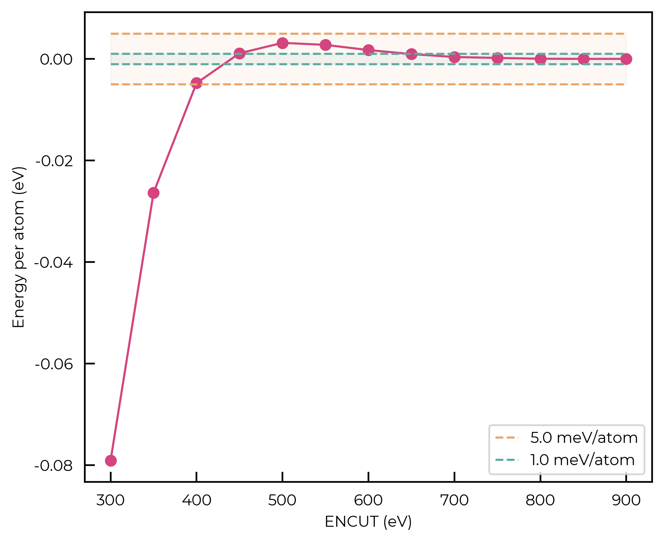
Typically, you converge these parameters to 1 meV/atom for high accuracy (highly recommended) and 5 meV/atom for moderate accuracy.
For this qualitative example, we’ll use a convergence threshold of 5 meV/atom. As shown in the plots below, this corresponds to a k-point mesh of 7x7x7 and a cutoff of 450 eV.
Convergence Plots for Host Structure
# Output from running vaspup2.0 `data-converge`
encut_results = """Directory:     Total Energy/eV: (per atom): Difference (meV/atom): Average Force Difference (meV/Å):
e300            -12.66773427    -6.3338671
e350            -12.56221754    -6.2811087        -52.7584                  0.0000
e400            -12.51904641    -6.2595232        -21.5855                  0.0000
e450            -12.50729263    -6.2536463        -5.8769                   0.0000
e500            -12.50319088    -6.2515954        -2.0509                   0.0000
e550            -12.50398209    -6.2519910        0.3956                    0.0000
e600            -12.50603059    -6.2530152        1.0242                    0.0000
e650            -12.50759882    -6.2537994        0.7842                    0.0000
e700            -12.50876680    -6.2543834        0.5840                    0.0000
e750            -12.50912904    -6.2545645        0.1811                    0.0000
e800            -12.50945676    -6.2547283        0.1638                    0.0000
e850            -12.50950670    -6.2547533        0.0250                    0.0000
e900            -12.50951238    -6.2547561        0.0028                    0.0000"""
We can parse the results using the following function parse_encut, which will return a plot of the convergence results.
import matplotlib.pyplot as plt
import numpy as np

def parse_encut(encut):
    """
    Parse and plot the ENCUT convergence results,
    generated by vaspup2.0 `data-converge` command.
    """
    # Get values from 3rd column into list
    energies_per_atom = np.array([float(line.split()[2]) for line in encut.split("\n")[1:]])
    normalised_energies_per_atom = energies_per_atom - energies_per_atom[-1]
    # Get encut values from 1st column into list
    encut_values = [int(line.split()[0][1:]) for line in encut.split("\n")[1:]]
    # return encut_values, encut_energies_per_atom

    # Plot
    fig, ax = plt.subplots(figsize=(6, 5), dpi=400)
    ax.plot(encut_values, normalised_energies_per_atom, marker="o", color="#D4447E")
    # Draw lines +- 5 meV/atom from the last point (our most accurate value)
    for threshold, color in zip([0.005, 0.001], ("#E9A66C", "#5FABA2")):
        ax.hlines(
            y=normalised_energies_per_atom[-1] + threshold,
            xmin=encut_values[0], xmax=encut_values[-1],
            color=color, linestyles="dashed",
            label=f"{1000*threshold} meV/atom"
        )
        ax.hlines(
            y=normalised_energies_per_atom[-1] - threshold,
            xmin=encut_values[0], xmax=encut_values[-1],
            color=color, linestyles="dashed",
        )
        # Fill the area between the lines
        ax.fill_between(
            encut_values,
            normalised_energies_per_atom[-1] - threshold,
            normalised_energies_per_atom[-1] + threshold,
            color=color, alpha=0.08,
        )
    # Add labels
    ax.set_xlabel("ENCUT (eV)")
    ax.set_ylabel("Energy per atom (eV)")
    ax.legend(frameon=True)
    return fig
fig = parse_encut(encut_results)
Idem for the kpoints:
kpoint_results = """Directory:     Total Energy/eV: (per atom): Difference (meV/atom): Average Force Difference (meV/Å):
k4,4,4          -12.58620794    -6.2931039
k5,5,5          -12.66431702    -6.3321585        39.0546                   0.0000
k6,6,6          -12.66659966    -6.3332998        1.1413                    0.0000
k7,7,7          -12.66180056    -6.3309002        -2.3996                   0.0000
k8,8,8          -12.64832289    -6.3241614        -6.7388                   0.0000
k9,9,9          -12.65998187    -6.3299909        5.8295                    0.0000
k_10,10,10      -12.66773427    -6.3338671        3.8762                    0.0000
k_11,11,11      -12.66360626    -6.3318031        -2.0640                   0.0000
k_12,12,12      -12.65463699    -6.3273184        -4.4847                   0.0000
k_13,13,13      -12.65957706    -6.3297885        2.4701                    0.0000
k_14,14,14      -12.66096859    -6.3304842        0.6957                    0.0000
k_15,15,15      -12.65856041    -6.3292802        -1.2040                   0.0000
k_16,16,16      -12.65562228    -6.3278111        -1.4691                   0.0000"""
def parse_kpoints(kpoints):
    """Function to parse kpoints convergence results from the string produced by vaspup2.0
    and plot them."""
    # Get values from 3rd column into list
    energies_per_atom = np.array([float(line.split()[2]) for line in kpoints.split("\n")[1:]])
    normalised_energies_per_atom = energies_per_atom - energies_per_atom[-1]
    # Get encut values from 1st column into list
    data = [line.split() for line in kpoints.split("\n")[1:]]
    kpoints_values = [line[0].split("k")[1].split("_")[-1].split()[0] for line in data]
    # print(kpoints_values)
    #return kpoints_values, kpoints_energies_per_atom
    # Plot
    fig, ax = plt.subplots(figsize=(6, 5), dpi=400)
    ax.plot(kpoints_values, normalised_energies_per_atom, marker="o", color="#D4447E")
    # Draw lines +- 5 meV/atom from the last point (our most accurate value)
    for threshold, color in zip([0.005, 0.001], ("#E9A66C", "#5FABA2")):
        ax.hlines(
            y=normalised_energies_per_atom[-1] + threshold,
            xmin=kpoints_values[0],
            xmax=kpoints_values[-1],
            color=color,
            linestyles="dashed",
            label=f"{1000*threshold} meV/atom"
        )
        ax.hlines(
            y=normalised_energies_per_atom[-1] - threshold,
            xmin=kpoints_values[0],
            xmax=kpoints_values[-1],
            color=color,
            linestyles="dashed",
        )
        # Fill the area between the lines
        ax.fill_between(
            kpoints_values,
            normalised_energies_per_atom[-1] - threshold,
            normalised_energies_per_atom[-1] + threshold,
            color=color,
            alpha=0.08,
        )
    # Add axis labels
    ax.set_xlabel("KPOINTS")
    ax.set_ylabel("Energy per atom (eV)")
    ax.set_xticks(range(len(kpoints_values)))
    ax.set_xticklabels(kpoints_values, rotation=90)  # Rotate xticks
    ax.legend(frameon=True)
    return fig
fig = parse_kpoints(kpoint_results)
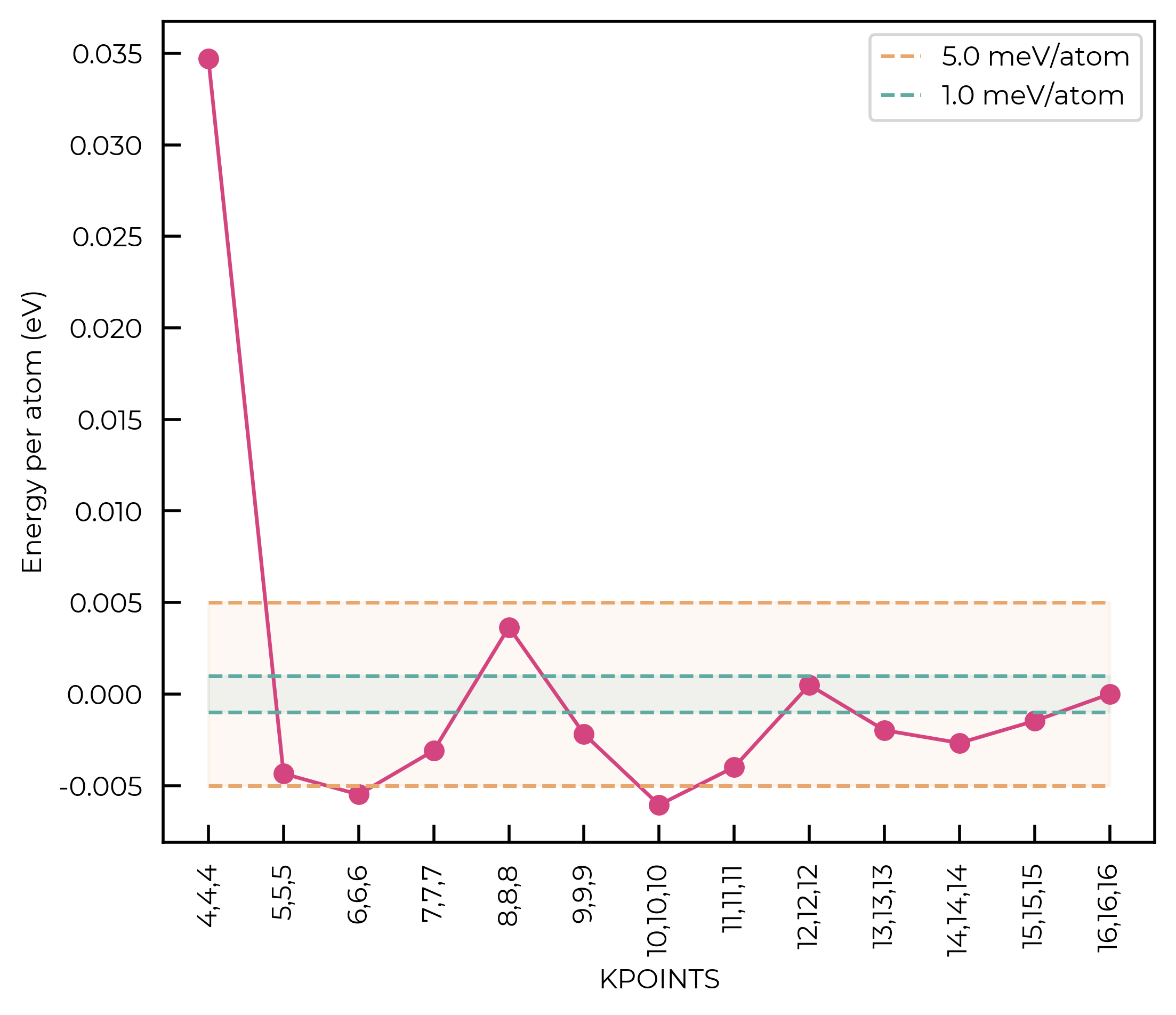
Converged values to 5 meV/atom: # Note that in a proper defect study, you’d converge to 1 meV/atom!
kpoints:
7x7x7cutoff:
450eV
2.2 Bulk Relaxation
Generate input files
We generate the VASP input files to relax the primitive structure:
For the POTCAR, we use the default VASP PBE pseudopotentials, which we read from doped:
from monty.serialization import loadfn
from pymatgen.core.structure import Structure

potcar_yaml = "../doped/VASP_sets/PotcarSet.yaml"
potcar_dict = loadfn(potcar_yaml)

if not prim_struc:
    prim_struc = Structure.from_file("MgO/Input_files/prim_struc_POSCAR")
print(f"Default PBE pseudopotentials:")
potcar_names = []
for el in prim_struc.elements:
    print(f"Element {el}: {potcar_dict['POTCAR'][str(el)]}")
    potcar_names.append(potcar_dict["POTCAR"][str(el)])
Default PBE pseudopotentials:
Element Mg: Mg
Element O: O
# Generate input files for VASP
from pymatgen.io.vasp.inputs import Incar, Poscar, Potcar, Kpoints, VaspInput

poscar = Poscar(prim_struc)
kpoints = Kpoints(kpts=((7,7,7),)) # Using converged kgrid from previous section
potcar = Potcar(
    potcar_names # Recommended VASP pseudopotentials for Mg, O
)  # comment out if running on Colab; need POTCAR directory setup with pymatgen
Finally, we load the INCAR file and update the ENCUT value. Note that because we’re relaxing the volume of the structure, we need to increase our converged ENCUT by 30% (see discussion of Pulay stress).
incar = Incar.from_file("./MgO/Input_files/INCAR_bulk_relax")
incar.update(
    {
        "ENCUT": 450 * 1.3, # Increase ENCUT by 30% because we're relaxing volume (Pulay stress)
        # Paralelisation
        "KPAR": 2,
        "NCORE": 8, # Might need updating for your HPC!
        # Functional
        "GGA": "PS",
        # Relaxation
        "IBRION": 2,
        "ISIF": 3, # Relax cell
        "NSW": 800, # Max number of steps
        # Accuracy and thresholds
        "ISYM": 2, # Symmetry on
        "PREC": "Accurate",
        "EDIFF": 1e-6, # Electronic convergence
        "EDIFFG": 1e-5, # Ionic convergence
        "ALGO": "Normal",
    }
)
incar
{'GGA': 'Ps', 'ALGO': 'Normal', 'EDIFF': 1e-06, 'EDIFFG': 1e-05, 'ENCUT': 585.0, 'IBRION': 2, 'ISIF': 3, 'ISMEAR': 0, 'ISPIN': 1, 'ISYM': 2, 'KPAR': 2, 'LCHARG': True, 'LHFCALC': False, 'LWAVE': False, 'NCORE': 8, 'NELM': 60, 'NELMIN': 5, 'NSW': 800, 'PREC': 'Accurate', 'SIGMA': 0.1}
In the INCAR, remember to adapt the KPAR and NCORE to values that are appropriate for your computer cluster!
vasp_input = VaspInput(incar, kpoints, poscar, potcar)
# vasp_input = VaspInput(incar, kpoints, poscar, potcar=["Mg", "O"], potcar_spec=True)  # -- use this instead for Colab
vasp_input.write_input("MgO/Bulk_relax")  # write to folder
We know submit the bulk relaxation in a computer cluster. After the first relaxation is converged, we resubmit with the converged ENCUT value (without increasing it by 30%), as we need to use the same ENCUT value for the bulk and defect calculations:
cp CONTCAR POSCAR
sed -i 's/ENCUT = 585/ENCUT = 450/g' INCAR
qsub -N bulk_relax job # Update for your HPC!
After the relaxation is complete, we parse the resulting vasprun.xml and CONTCAR to the current directory.
# We can check the volume change upon relaxation like this:
from pymatgen.core.structure import Structure

s_poscar = Structure.from_file("MgO/Bulk_relax/POSCAR")
s_contcar = Structure.from_file("MgO/Bulk_relax/CONTCAR")
s_poscar.volume, s_contcar.volume
(18.442770099568843, 18.521290988527692)
from pymatgen.io.vasp.outputs import Vasprun
import os

# Can check if relaxation is converged by parsing the vasprun.xml
if os.path.exists("MgO/Bulk_relax/vasprun.xml"):
    vr = Vasprun("MgO/Bulk_relax/vasprun.xml")
elif os.path.exists("MgO/Bulk_relax/vasprun.xml.gz"):
    vr = Vasprun("MgO/Bulk_relax/vasprun.xml.gz")
else:
    raise FileNotFoundError("No vasprun.xml found in the Bulk_relax directory")
print(f"Relaxation converged?", vr.converged)
Relaxation converged? True
3. Generate defects
Load the bulk relaxed structure:
from pymatgen.core.structure import Structure
from doped.utils.symmetry import get_primitive_structure

if not os.path.exists("./MgO/Bulk_relax/CONTCAR"):
    print("Please run the bulk relaxation first!")
else:
    prim_struc = get_primitive_structure(Structure.from_file("./MgO/Bulk_relax/CONTCAR"))
We can generate all the intrinsic defects for that bulk structure by running the DefectsGenerator class:
from doped.generation import DefectsGenerator
# generate all intrinsic defects, enforcing the use of a cubic supercell in this example case:
defect_gen = DefectsGenerator(structure=prim_struc, supercell_gen_kwargs={"force_cubic":True})
Guessing charge states: 100.0%|██████████| [00:01, 95.85it/s]
Vacancies    Guessed Charges    Conv. Cell Coords    Wyckoff
-----------  -----------------  -------------------  ---------
v_Mg         [+1,0,-1,-2]       [0.000,0.000,0.000]  4a
v_O          [+2,+1,0,-1]       [0.500,0.500,0.500]  4b

Substitutions    Guessed Charges    Conv. Cell Coords    Wyckoff
---------------  -----------------  -------------------  ---------
Mg_O             [+4,+3,+2,+1,0]    [0.500,0.500,0.500]  4b
O_Mg             [0,-1,-2,-3,-4]    [0.000,0.000,0.000]  4a

Interstitials    Guessed Charges    Conv. Cell Coords    Wyckoff
---------------  -----------------  -------------------  ---------
Mg_i_Td          [+2,+1,0]          [0.250,0.250,0.250]  8c
O_i_Td           [0,-1,-2]          [0.250,0.250,0.250]  8c

The number in the Wyckoff label is the site multiplicity/degeneracy of that defect in the conventional ('conv.') unit cell, which comprises 4 formula unit(s) of MgO.
Note that you can check the documentation of this class by running DefectsGenerator?:
from doped.generation import DefectsGenerator
DefectsGenerator?
Init signature:
DefectsGenerator(
    structure: 'Structure | Atoms | PathLike',
    extrinsic: str | list | dict | None = None,
    interstitial_coords: list | None = None,
    generate_supercell: bool = True,
    charge_state_gen_kwargs: dict | None = None,
    supercell_gen_kwargs: dict[str, int | float | bool] | None = None,
    interstitial_gen_kwargs: dict | bool | None = None,
    target_frac_coords: list | None = None,
    processes: int | None = None,
    **kwargs,
)
Docstring:      Class for generating ``doped`` |DefectEntry| objects.
Init docstring:
Generates ``doped`` |DefectEntry| objects for defects in the input host
structure. By default, generates all intrinsic defects, but extrinsic
defects (impurities) can also be created using the ``extrinsic``
argument.

Interstitial sites are generated using Voronoi tessellation by default
(found to be the most reliable) using the ``get_interstitial_sites``
function, which also generates adsorbate sites if the structure is
determined to be a slab/layer/rod. This can be controlled using the
``interstitial_gen_kwargs`` argument. Alternatively, a list of
interstitial sites (or single interstitial site) can be manually
specified using the ``interstitial_coords`` argument.

By default, supercells are generated for each defect using the
``doped`` ``get_ideal_supercell_matrix()`` function (see docstring),
with default settings of ``min_image_distance = 10`` (minimum distance
between periodic images of 10 Å), ``min_atoms = 50`` (minimum 50 atoms
in the supercell) and ``ideal_threshold = 0.1`` (allow up to 10% larger
supercell if it is a diagonal expansion of the primitive or
conventional cell). This uses a custom algorithm in ``doped`` to
efficiently search over possible supercell transformations and identify
that with the minimum number of atoms (hence computational cost) that
satisfies the minimum image distance, number of atoms and
``ideal_threshold`` constraints. These settings can be controlled by
specifying keyword arguments with ``supercell_gen_kwargs``, which are
passed to ``get_ideal_supercell_matrix()`` (e.g. for a minimum image
distance of 15 Å with at least 100 atoms, ``supercell_gen_kwargs``
would be: ``{'min_image_distance': 15, 'min_atoms': 100}``). If the
input structure already satisfies these constraints (for the same
number of atoms as the ``doped``-generated supercell), then it will be
used. Alternatively if ``generate_supercell = False``, then no
supercell is generated and the input structure is used as the defect &
bulk supercell. (Note this may give a slightly different (but fully
equivalent) set of coordinates).

The algorithm for determining defect entry names is to use the
``pymatgen`` defect name (e.g. ``v_Cd``, ``Cd_Te`` etc.) for vacancies
/ antisites / substitutions, unless there are multiple inequivalent
sites for the defect, in which case the point group of the defect site
is appended (e.g. ``v_Cd_Td``, ``Cd_Te_Td`` etc.), and if this is still
not unique, then element identity and distance to the nearest neighbour
of the defect site is appended (e.g. ``v_Cd_Td_Te2.83``,
``Cd_Te_Td_Cd2.83`` etc.). For interstitials, the same naming scheme is
used, but the point group is always appended to the ``pymatgen`` name.

Possible charge states for the defects are estimated using the
probability of the corresponding defect element oxidation state, the
magnitude of the charge state, and the maximum magnitude of the host
oxidation states (i.e. how 'charged' the host is). Large (absolute)
charge states, low probability oxidation states and/or greater
charge/oxidation state magnitudes than that of the host are
disfavoured. This can be controlled using the ``probability_threshold``
(default = 0.0075) or ``padding`` (default = 1) keys in the
``charge_state_gen_kwargs`` parameter, which are passed to the
``guess_defect_charge_states()`` function. The input and computed
values used to guess charge state probabilities are provided in the
``DefectEntry.charge_state_guessing_log`` attributes. See docs for
examples of modifying the generated charge states, and the docstrings
of ``charge_state_probability()`` & ``get_vacancy_charge_states()`` for
more details on the charge state guessing algorithm. The ``doped``
algorithm was found to give optimal performance in terms of efficiency
and completeness (see JOSS paper), but of course may not be perfect in
all cases, so make sure to critically consider the estimated charge
states for your system!

Note that Wyckoff letters can depend on the ordering of elements in the
conventional standard structure, for which doped uses the ``spglib``
convention.

Args:
    structure (|Structure|):
        Structure of the host material, either as a ``pymatgen``
        |Structure|, ``ASE`` |Atoms| or path to a structure file
        (e.g. ``CONTCAR``). If this is not the primitive unit cell, it
        will be reduced to the primitive cell for defect generation,
        before supercell generation.
    extrinsic (str | list | dict):
        List or dict of elements (or string for single element) to be
        used for extrinsic defect generation (i.e. dopants/impurities).
        If a list is provided, all possible substitutional defects for
        each extrinsic element will be generated. If a dict is
        provided, the keys should be the host elements to be
        substituted, and the values the extrinsic element(s) to
        substitute in; as a string or list. In both cases, all possible
        extrinsic interstitials are generated.
    interstitial_coords (list):
        List of fractional coordinates (corresponding to the input
        structure), or a single set of fractional coordinates, to use
        as interstitial defect site(s). Default (when
        ``interstitial_coords`` not specified) is to automatically
        generate interstitial sites using Voronoi tessellation.
        The input ``interstitial_coords`` are converted to
        ``DefectsGenerator.prim_interstitial_coords_mult_and_equiv_coords``,
        which are the corresponding fractional coordinates in
        ``DefectsGenerator.primitive_structure`` (which is used for
        defect generation), along with the multiplicity and equivalent
        coordinates, sorted according to the ``doped`` convention.
    generate_supercell (bool):
        Whether to generate a supercell for the output defect entries
        (using the custom algorithm in ``doped`` which efficiently
        searches over possible supercell transformations and identifies
        that with the minimum number of atoms (hence computational
        cost) that satisfies the minimum image distance, number of
        atoms and ``ideal_threshold`` constraints -- which can be
        controlled with ``supercell_gen_kwargs``).
        If ``False``, then the input structure is used as the defect &
        bulk supercell (note this may give a slightly different (but
        fully equivalent) set of coordinates).
        Default is ``True``.
    charge_state_gen_kwargs (dict):
        Keyword arguments to pass to the ``guess_defect_charge_states``
        function (such as ``probability_threshold`` (default = 0.0075,
        used for substitutions and interstitials) and ``padding``
        (default = 1, used for vacancies)) to control defect charge
        state generation.
    supercell_gen_kwargs (dict):
        Keyword arguments to pass to the ``get_ideal_supercell_matrix``
        function (such as ``min_image_distance`` (default = 10),
        ``min_atoms`` (default = 50), ``ideal_threshold`` (default =
        0.1), ``force_cubic`` -- which enforces a (near-)cubic
        supercell output (default = False), or ``force_diagonal``
        (default = False)).
    interstitial_gen_kwargs (dict, bool):
        Keyword arguments to be passed to
        :func:`~doped.generation.get_interstitial_sites()` (such as
        ``min_dist`` (0.9 Å, or 0.5 Å for Hydrogen), ``clustering_tol``
        (0.8 Å), ``symm_pref_dist_factor`` (0.85), ``stol`` (0.32),
        ``tight_stol`` (0.02), ``symprec`` (0.01), ``vacuum_radius``
        (1.5 * bulk bond length), ``include_unique_wyckoffs`` (False)
        -- see its docstring, parentheses indicate default values), or
        ``InterstitialGenerator`` (where only ``min_dist`` is used) if
        ``interstitial_coords`` is specified. If set to ``False``,
        interstitial generation will be skipped entirely.
    target_frac_coords (list):
        Defects are placed at the closest equivalent site to these
        fractional coordinates in the generated supercells. Default is
        ``[0.5, 0.5, 0.5]`` (i.e. the supercell centre, to aid
        visualisation).
    processes (int):
        Number of processes to use for multiprocessing. If not set,
        defaults to one less than the number of CPUs available.
    **kwargs:
        Additional keyword arguments for defect generation. Options:

        - ``{defect}_elements`` where ``{defect}`` is ``vacancy``,
          ``substitution``, or ``interstitial``, in which cases only
          those defects of the specified elements will be generated
          (where ``{defect}_elements`` is a list of element symbol
          strings). Setting ``{defect}_elements`` to an empty list will
          skip defect generation for that defect type entirely.
        - ``{defect}_charge_states`` to specify the charge states to use
          for all defects of that type (as a list of integers).
        - ``neutral_only`` to only generate neutral charge states.
        - ``symprec`` for ``get_sga_and_symprec()``,
          ``get_primitive_structure``, defect object initialisation
          etc. Default is ``0.01``.
        - Keyword arguments for ``get_all_equiv_sites``, such as
          ``dist_tol_factor``, ``fixed_symprec_and_dist_tol_factor``,
          and ``verbose``.

Key attributes:
    defect_entries (dict):
        Dictionary of ``{defect_species: DefectEntry}`` for all defect
        entries (with charge state and supercell properties) generated.
    defects (dict):
        Dictionary of ``{defect_type: [Defect, ...]}`` for all defect
        objects generated.
    primitive_structure (|Structure|):
        Primitive cell structure of the host used to generate defects.
    supercell_matrix (Matrix):
        Matrix to generate defect/bulk supercells from the primitive
        cell structure.
    bulk_supercell (|Structure|):
        Supercell structure of the host (equal to
        ``self.primitive_structure * self.supercell_matrix``).
    conventional_structure (|Structure|):
        Conventional cell structure of the host according to the Bilbao
        Crystallographic Server (BCS) definition, used to determine
        defect site Wyckoff labels and multiplicities.
    prim_interstitial_coords_mult_and_equiv_coords (list):
        List of interstitial coordinates in the primitive cell, their
        multiplicity and the equivalent fractional coordinates, as a
        list of tuples.

    |DefectsGenerator| input parameters are also set as attributes.
File:           ~/Packages/doped/doped/generation.py
Type:           type
Subclasses:
Can check the dimensions of the generated supercell by calling the bulk_supercell method:
defect_gen.bulk_supercell.lattice
Lattice
    abc : 12.599839224 12.599839224 12.599839224
 angles : 90.0 90.0 90.0
 volume : 2000.2994265838051
      A : 12.599839224 -4.440892098500626e-16 -4.440892098500626e-16
      B : -4.440892098500626e-16 12.599839224 4.440892098500626e-16
      C : 4.440892098500626e-16 4.440892098500626e-16 12.599839224
    pbc : True True True
which corresponds to the following expansion of the primitive cell:
defect_gen.supercell_matrix
array([[-3,  3,  3],
       [ 3, -3,  3],
       [ 3,  3, -3]])
We can see the generated Defect objects by calling the defects method:
defect_gen.defects
{'vacancies': [v_Mg vacancy defect at site [0.000,0.000,0.000] in structure,
  v_O vacancy defect at site [0.500,0.500,0.500] in structure],
 'substitutions': [Mg_O substitution defect at site [0.500,0.500,0.500] in structure,
  O_Mg substitution defect at site [0.000,0.000,0.000] in structure],
 'interstitials': [Mg_i interstitial defect at site [0.250,0.250,0.250] in structure,
  O_i interstitial defect at site [0.250,0.250,0.250] in structure]}
And the associated DefectEntry keys by calling the defect_entries method:
# Names of generated defects with their charges
defect_gen.defect_entries.keys()
dict_keys(['v_Mg_+1', 'v_Mg_0', 'v_Mg_-1', 'v_Mg_-2', 'v_O_+2', 'v_O_+1', 'v_O_0', 'v_O_-1', 'Mg_O_+4', 'Mg_O_+3', 'Mg_O_+2', 'Mg_O_+1', 'Mg_O_0', 'O_Mg_0', 'O_Mg_-1', 'O_Mg_-2', 'O_Mg_-3', 'O_Mg_-4', 'Mg_i_Td_+2', 'Mg_i_Td_+1', 'Mg_i_Td_0', 'O_i_Td_0', 'O_i_Td_-1', 'O_i_Td_-2'])
In this tutorial, we’ll only consider the Mg substitution (Mg_O in the table above):
defect_gen.defects = {
    "substitutions": [
    defect for defect in defect_gen.defects["substitutions"] if defect.name == "Mg_O"], # select Mg_O
}
defect_gen.defect_entries = {
    k: v for k, v in defect_gen.defect_entries.items() if "Mg_O" in k
}
If we wanted to manually add some extra charge states (e.g. some positive charge states for Mg_O), we
can do so using the add_charge_states method:
defect_gen.add_charge_states("Mg_O", [-1, ])
# Check that now we only have the O interstitial
defect_gen.defect_entries.keys()
dict_keys(['Mg_O_+4', 'Mg_O_+3', 'Mg_O_+2', 'Mg_O_+1', 'Mg_O_0'])
And we can save it to a json file for later use:
defect_gen.to_json("MgO/defect_gen.json.gz")
Which we can later reload using the from_json method:
from doped.generation import DefectsGenerator
# Load from JSON
defect_gen = DefectsGenerator.from_json("MgO/defect_gen.json.gz")
4. Determining the ground-state defect structures
At this point, it’s recommended that you use the ShakeNBreak approach to quickly identify the groundstate structures of your defects (or any alternative global optimisation method), before continuing on with the formation energy calculation workflow below. As detailed in the theory paper, skipping this step can result in drastically incorrect formation energies, transition levels, carrier capture (basically any property associated with defects). This approach is followed below, with a more in-depth explanation and tutorial given on the ShakeNBreak website.
Tip
See the main generation tutorial for notes on ShakeNBreak, and recommended workflow if skipping this step for any reason.
4.1 Generate distorted structures
To generate our distorted defect structures with ShakeNBreak (SnB), we can directly input our DefectsGenerator object to the SnB Distortions class:
from shakenbreak.input import Distortions
Dist = Distortions(defect_entries = defect_gen)
Oxidation states were not explicitly set, thus have been guessed as {'Mg': 2, 'O': -2}. If this is unreasonable you should manually set oxidation_states
Important
As with the doped functions, ShakeNBreak has been built and optimised to adopt reasonable defaults that work well for most host materials, however there is again a lot of customisation and control available, and you should carefully consider the appropriate settings and choices for your system. The ShakeNBreak workflow is shown in more detail in the\n”, SnB Python API tutorial on the SnB docs, and here we just show a brief example of the main steps.
Generating VASP input files for the trial distorted structures
defects_dict, distortion_metadata = Dist.write_vasp_files(
    output_path="MgO/SnB",
    # Update INCAR settings to not use GGA and NCORE according to your HPC cluster:
    user_incar_settings={
        # Functional:
        "GGA": "PS",
        "LHFCALC": False,
        "AEXX": 0.0,
        "HFSCREEN": 0.0,
        # Parallelisation:
        "NCORE": 8 # Might need updating for your HPC!
    },
    verbose=False,  # quiet output, set to True for info on generated structures!
)
Generating distorted defect structures...100.0%|██████████| [00:02, 2.53s/it]
Our distorted structures and VASP input files have now been generated in the folders with names matching the doped naming scheme:
!cat ./MgO/SnB/Mg_O_0/Bond_Distortion_-10.0%/INCAR
# MAY WANT TO CHANGE NCORE, KPAR, AEXX, ENCUT, IBRION, LREAL, NUPDOWN, ISPIN, MAGMOM = Typical variable parameters
# SHAKENBREAK INCAR WITH COARSE SETTINGS TO MAXIMISE SPEED WITH SUFFICIENT ACCURACY FOR QUALITATIVE STRUCTURE SEARCHING =
AEXX = 0.0
ALGO = Normal  # change to all if zhegv, fexcp/f or zbrent errors encountered (done automatically by snb-run)
EDIFF = 1e-05
EDIFFG = -0.01
ENCUT = 300.0
GGA = Ps
HFSCREEN = 0.0
IBRION = 2
ICHARG = 1
ICORELEVEL = 0
ISEARCH = 1
ISIF = 2
ISMEAR = 0
ISPIN = 2
ISYM = 0
LASPH = True
LCHARG = False
LHFCALC = False
LORBIT = 11
LREAL = Auto
LVHAR = True
LWAVE = False
NCORE = 8
NEDOS = 3000
NELM = 40
NSW = 300
NUPDOWN = 0.0
PREC = Accurate
ROPT = 0.001 0.001
SIGMA = 0.05
4.2 Send to HPCs and run relaxations
Can use the snb-run CLI function to quickly run calculations; see the Submitting the geometry optimisations section of the SnB CLI tutorial for this.
After the relaxations finish, you can use can parse the energies obtained by running the snb-parse -a command from the top-level folder containing your defect folders (e.g. Mg_O_0 etc. (with subfolders: Mg_O_0/Bond_Distortion_10.0% etc.)). This will parse the energies and store them in a Mg_O_0.yaml etc file in the defect folders, to allow easy plotting and analysis.
When can copy these files and the relaxed structures (CONTCARs) to our local PC with the following code:
shopt -s extglob # ensure extended globbing (pattern matching) is enabled
for defect in ./*{_,_-}[0-9]/; do cd $defect;
scp {remote_machine}:{path to ShakeNBreak folders}/${defect}${defect%?}.yaml .;
for distortion in (Bond_Distortion|Unperturbed|Rattled)*/;
do scp {remote_machine}:{path to ShakeNBreak folders}/${defect}${distortion}CONTCAR ${distortion};
done; cd ..; done
4.3 Analyse results
Plot final energies versus the applied distortion
To see if SnB found any energy-lowering distortions, we can plot the results using the functions in shakenbreak.plotting.
from importlib_metadata import version
version('shakenbreak')
'3.4.3'
from shakenbreak import energy_lowering_distortions, plotting
!cp -r MgO/SnB/Pre_Calculated_Results/* MgO/SnB/  # add our pre-calculated results
# skip this if you have run the calculations yourself!
defect_charges_dict = energy_lowering_distortions.read_defects_directories(output_path="MgO/SnB")
low_energy_defects = energy_lowering_distortions.get_energy_lowering_distortions(defect_charges_dict, output_path="MgO/SnB")
Mg_O
Mg_O_+3: Energy difference between minimum, found with 0.6 bond distortion, and unperturbed: -1.41 eV.
Energy lowering distortion found for Mg_O with charge +3. Adding to low_energy_defects dictionary.
Mg_O_+4: Energy difference between minimum, found with Rattled bond distortion, and unperturbed: -1.41 eV.
New (according to structure matching) low-energy distorted structure found for Mg_O_+4, adding to low_energy_defects['Mg_O'] list.
Mg_O_+2: Energy difference between minimum, found with 0.6 bond distortion, and unperturbed: -1.23 eV.
Low-energy distorted structure for Mg_O_+2 already found with charge states ['+3'], storing together.
Mg_O_0: Energy difference between minimum, found with 0.4 bond distortion, and unperturbed: -1.02 eV.
Low-energy distorted structure for Mg_O_0 already found with charge states ['+3', '+2'], storing together.
Mg_O_+1: Energy difference between minimum, found with 0.4 bond distortion, and unperturbed: -0.99 eV.
Low-energy distorted structure for Mg_O_+1 already found with charge states ['+3', '+2', '0'], storing together.

Comparing and pruning defect structures across charge states...
low_energy_defects is a dictionary of defects for which bond distortion found an energy-lowering reconstruction (which is missed with normal unperturbed relaxation), of the form {defect: [list of
distortion dictionaries (with corresponding charge states,
energy lowering, distortion factors, structures and charge
states for which these structures weren’t found)]}:
low_energy_defects.keys() # Show defect keys in dict
dict_keys(['Mg_O'])
low_energy_defects["Mg_O"][0].keys(), low_energy_defects["Mg_O"][0]
(dict_keys(['charges', 'structures', 'energy_diffs', 'bond_distortions', 'excluded_charges']),
 {'charges': [3, 2, 0, 1],
  'structures': [Structure Summary
   Lattice
       abc : 12.599837999999998 12.599837999999998 12.599837999999998
    angles : 90.0 90.0 90.0
    volume : 2000.2988436320181
         A : 12.599837999999998 4e-16 4e-16
         B : 4e-16 12.599837999999998 -4e-16
         C : -4e-16 -4e-16 12.599837999999998
       pbc : True True True
   PeriodicSite: Mg (8.42, -0.008923, -0.02327) [0.6682, -0.0007082, -0.001847]
   PeriodicSite: Mg (10.52, 2.086, -0.02451) [0.8347, 0.1655, -0.001945]
   PeriodicSite: Mg (10.52, -0.01224, 2.072) [0.8346, -0.0009711, 0.1644]
   PeriodicSite: Mg (4.205, -0.008532, 12.58) [0.3338, -0.0006771, 0.9981]
   PeriodicSite: Mg (6.314, 2.08, -0.0203) [0.5011, 0.1651, -0.001611]
   PeriodicSite: Mg (8.421, 4.179, 12.59) [0.6683, 0.3317, 0.9993]
   PeriodicSite: Mg (10.53, 6.291, 12.59) [0.8357, 0.4993, 0.9996]
   PeriodicSite: Mg (6.312, -0.02705, 2.058) [0.501, -0.002147, 0.1634]
   PeriodicSite: Mg (8.423, 2.078, 2.066) [0.6685, 0.1649, 0.164]
   PeriodicSite: Mg (10.52, 4.181, 2.066) [0.8351, 0.3319, 0.164]
   PeriodicSite: Mg (8.422, -0.03152, 4.166) [0.6684, -0.002501, 0.3307]
   PeriodicSite: Mg (10.52, 2.078, 4.166) [0.8352, 0.1649, 0.3306]
   PeriodicSite: Mg (10.53, -0.02719, 6.276) [0.8358, -0.002158, 0.4981]
   PeriodicSite: Mg (0.01233, -0.00832, -0.02374) [0.0009789, -0.0006604, -0.001884]
   PeriodicSite: Mg (2.108, 2.088, -0.02424) [0.1673, 0.1657, -0.001924]
   PeriodicSite: Mg (4.207, 4.186, 12.59) [0.3339, 0.3323, 0.9993]
   PeriodicSite: Mg (6.315, 6.294, 0.03391) [0.5012, 0.4995, 0.002691]
   PeriodicSite: Mg (8.422, 8.401, -0.0007354) [0.6684, 0.6668, -5.836e-05]
   PeriodicSite: Mg (10.52, 10.5, -0.0199) [0.8346, 0.833, -0.00158]
   PeriodicSite: Mg (2.106, -0.007372, 2.071) [0.1672, -0.0005851, 0.1644]
   PeriodicSite: Mg (4.202, 2.085, 2.066) [0.3335, 0.1654, 0.1639]
   PeriodicSite: Mg (6.315, 4.168, 2.054) [0.5012, 0.3308, 0.163]
   PeriodicSite: Mg (8.43, 6.292, 2.066) [0.669, 0.4994, 0.164]
   PeriodicSite: Mg (10.51, 8.398, 2.076) [0.8343, 0.6665, 0.1647]
   PeriodicSite: Mg (4.2, -0.02279, 4.167) [0.3333, -0.001808, 0.3307]
   PeriodicSite: Mg (6.309, 1.981, 4.092) [0.5007, 0.1572, 0.3248]
   PeriodicSite: Mg (8.461, 4.184, 4.128) [0.6715, 0.3321, 0.3276]
   PeriodicSite: Mg (10.52, 6.292, 4.158) [0.8351, 0.4994, 0.33]
   PeriodicSite: Mg (6.314, 12.53, 6.274) [0.5012, 0.9947, 0.4979]
   PeriodicSite: Mg (8.497, 1.981, 6.28) [0.6743, 0.1572, 0.4984]
   PeriodicSite: Mg (10.53, 4.168, 6.273) [0.8361, 0.3308, 0.4979]
   PeriodicSite: Mg (8.421, -0.02357, 8.389) [0.6684, -0.001871, 0.6658]
   PeriodicSite: Mg (10.52, 2.084, 8.386) [0.8352, 0.1654, 0.6656]
   PeriodicSite: Mg (10.52, -0.00747, 10.48) [0.8347, -0.0005928, 0.8319]
   PeriodicSite: Mg (0.01183, 4.185, 12.58) [0.0009386, 0.3321, 0.9981]
   PeriodicSite: Mg (2.101, 6.294, -0.02034) [0.1667, 0.4995, -0.001614]
   PeriodicSite: Mg (4.2, 8.4, -0.008791) [0.3333, 0.6667, -0.0006977]
   PeriodicSite: Mg (6.312, 10.51, -0.004808) [0.5009, 0.8341, -0.0003816]
   PeriodicSite: Mg (0.01297, 2.086, 2.071) [0.001029, 0.1656, 0.1644]
   PeriodicSite: Mg (2.105, 4.182, 2.066) [0.167, 0.3319, 0.1639]
   PeriodicSite: Mg (4.188, 6.295, 2.054) [0.3324, 0.4996, 0.163]
   PeriodicSite: Mg (6.313, 8.41, 2.066) [0.501, 0.6674, 0.164]
   PeriodicSite: Mg (8.418, 10.49, 2.076) [0.6681, 0.8327, 0.1648]
   PeriodicSite: Mg (0.0118, -0.00859, 4.168) [0.0009368, -0.0006817, 0.3308]
   PeriodicSite: Mg (2.108, 2.088, 4.168) [0.1673, 0.1657, 0.3308]
   PeriodicSite: Mg (4.208, 4.188, 4.152) [0.334, 0.3323, 0.3295]
   PeriodicSite: Mg (6.319, 6.298, 4.042) [0.5015, 0.4999, 0.3208]
   PeriodicSite: Mg (8.415, 8.395, 4.173) [0.6679, 0.6663, 0.3312]
   PeriodicSite: Mg (10.51, 10.49, 4.169) [0.8343, 0.8327, 0.3309]
   PeriodicSite: Mg (2.101, -0.01162, 6.274) [0.1667, -0.0009219, 0.4979]
   PeriodicSite: Mg (4.197, 2.026, 6.271) [0.3331, 0.1608, 0.4977]
   PeriodicSite: Mg (6.536, 3.742, 6.054) [0.5188, 0.297, 0.4805]
   PeriodicSite: Mg (8.546, 6.298, 6.27) [0.6783, 0.4998, 0.4976]
   PeriodicSite: Mg (10.52, 8.41, 6.276) [0.8351, 0.6675, 0.4981]
   PeriodicSite: Mg (4.206, -0.02298, 8.382) [0.3338, -0.001824, 0.6652]
   PeriodicSite: Mg (6.318, 2.025, 8.391) [0.5014, 0.1608, 0.666]
   PeriodicSite: Mg (8.437, 4.187, 8.38) [0.6697, 0.3323, 0.6651]
   PeriodicSite: Mg (10.53, 6.295, 8.4) [0.8361, 0.4996, 0.6667]
   PeriodicSite: Mg (6.314, 12.59, 10.49) [0.5011, 0.999, 0.8323]
   PeriodicSite: Mg (8.42, 2.087, 10.48) [0.6682, 0.1657, 0.8318]
   PeriodicSite: Mg (10.52, 4.182, 10.48) [0.8352, 0.3319, 0.832]
   PeriodicSite: Mg (0.01177, 8.399, -0.02368) [0.0009345, 0.6666, -0.00188]
   PeriodicSite: Mg (2.106, 10.5, -0.02466) [0.1672, 0.833, -0.001957]
   PeriodicSite: Mg (12.59, 6.292, 2.058) [0.9995, 0.4993, 0.1633]
   PeriodicSite: Mg (2.098, 8.402, 2.065) [0.1665, 0.6669, 0.1639]
   PeriodicSite: Mg (4.202, 10.5, 2.066) [0.3335, 0.8335, 0.164]
   PeriodicSite: Mg (-0.00281, 4.18, 4.167) [-0.000223, 0.3317, 0.3307]
   PeriodicSite: Mg (2.002, 6.289, 4.092) [0.1589, 0.4991, 0.3248]
   PeriodicSite: Mg (4.205, 8.44, 4.128) [0.3337, 0.6698, 0.3276]
   PeriodicSite: Mg (6.312, 10.5, 4.158) [0.501, 0.8335, 0.33]
   PeriodicSite: Mg (0.00894, 2.081, 6.274) [0.0007095, 0.1651, 0.4979]
   PeriodicSite: Mg (2.047, 4.177, 6.271) [0.1624, 0.3315, 0.4977]
   PeriodicSite: Mg (3.762, 6.516, 6.054) [0.2986, 0.5172, 0.4805]
   PeriodicSite: Mg (6.319, 8.526, 6.27) [0.5015, 0.6767, 0.4976]
   PeriodicSite: Mg (8.43, 10.5, 6.276) [0.6691, 0.8335, 0.4981]
   PeriodicSite: Mg (0.01186, -0.008531, 8.383) [0.000941, -0.0006771, 0.6653]
   PeriodicSite: Mg (2.093, 2.073, 8.38) [0.1661, 0.1645, 0.6651]
   PeriodicSite: Mg (4.129, 4.108, 8.458) [0.3277, 0.3261, 0.6713]
   PeriodicSite: Mg (6.534, 6.513, 8.824) [0.5186, 0.5169, 0.7003]
   PeriodicSite: Mg (8.46, 8.439, 8.384) [0.6715, 0.6698, 0.6654]
   PeriodicSite: Mg (10.52, 10.5, 8.387) [0.8351, 0.8335, 0.6656]
   PeriodicSite: Mg (2.108, 12.59, 10.48) [0.1673, 0.9994, 0.8318]
   PeriodicSite: Mg (4.208, 2.073, 10.49) [0.334, 0.1645, 0.8329]
   PeriodicSite: Mg (6.317, 4.176, 10.54) [0.5014, 0.3315, 0.8367]
   PeriodicSite: Mg (8.496, 6.288, 10.59) [0.6743, 0.4991, 0.8402]
   PeriodicSite: Mg (10.52, 8.402, 10.49) [0.8352, 0.6669, 0.8326]
   PeriodicSite: Mg (0.00809, 10.5, 2.072) [0.000642, 0.833, 0.1644]
   PeriodicSite: Mg (-0.01129, 8.402, 4.166) [-0.0008957, 0.6668, 0.3306]
   PeriodicSite: Mg (2.098, 10.5, 4.165) [0.1665, 0.8335, 0.3306]
   PeriodicSite: Mg (-0.04604, 6.294, 6.274) [-0.003654, 0.4996, 0.4979]
   PeriodicSite: Mg (2.001, 8.476, 6.28) [0.1588, 0.6727, 0.4984]
   PeriodicSite: Mg (4.188, 10.51, 6.273) [0.3324, 0.8345, 0.4978]
   PeriodicSite: Mg (-0.002179, 4.186, 8.382) [-0.0001729, 0.3322, 0.6652]
   PeriodicSite: Mg (2.046, 6.297, 8.391) [0.1624, 0.4998, 0.666]
   PeriodicSite: Mg (4.208, 8.417, 8.38) [0.3339, 0.6681, 0.6651]
   PeriodicSite: Mg (6.315, 10.51, 8.4) [0.5012, 0.8345, 0.6667]
   PeriodicSite: Mg (0.01268, 2.088, 10.48) [0.001006, 0.1657, 0.8318]
   PeriodicSite: Mg (2.093, 4.188, 10.5) [0.1661, 0.3324, 0.8329]
   PeriodicSite: Mg (4.197, 6.297, 10.54) [0.3331, 0.4998, 0.8366]
   PeriodicSite: Mg (6.309, 8.475, 10.59) [0.5007, 0.6726, 0.8402]
   PeriodicSite: Mg (8.423, 10.5, 10.49) [0.6685, 0.8335, 0.8326]
   PeriodicSite: Mg (-0.006919, 10.51, 6.276) [-0.0005491, 0.8341, 0.4981]
   PeriodicSite: Mg (-0.003016, 8.4, 8.388) [-0.0002393, 0.6667, 0.6658]
   PeriodicSite: Mg (2.104, 10.5, 8.386) [0.167, 0.8335, 0.6656]
   PeriodicSite: Mg (0.008326, 6.294, 10.49) [0.0006608, 0.4995, 0.8324]
   PeriodicSite: Mg (2.108, 8.399, 10.48) [0.1673, 0.6666, 0.8318]
   PeriodicSite: Mg (4.202, 10.5, 10.48) [0.3335, 0.8335, 0.8321]
   PeriodicSite: Mg (0.01287, 10.5, 10.48) [0.001022, 0.8331, 0.8319]
   PeriodicSite: Mg (5.586, 5.565, 6.999) [0.4433, 0.4417, 0.5555]
   PeriodicSite: O (10.51, 2.091, 2.078) [0.8341, 0.1659, 0.165]
   PeriodicSite: O (0.015, 4.191, 2.077) [0.00119, 0.3327, 0.1648]
   PeriodicSite: O (0.01716, 2.094, 4.179) [0.001362, 0.1662, 0.3316]
   PeriodicSite: O (6.312, 2.082, 2.069) [0.5009, 0.1653, 0.1642]
   PeriodicSite: O (8.411, 4.189, 2.079) [0.6675, 0.3325, 0.165]
   PeriodicSite: O (10.5, 6.287, 2.083) [0.8337, 0.499, 0.1653]
   PeriodicSite: O (0.008883, 8.389, 2.077) [0.000705, 0.6658, 0.1649]
   PeriodicSite: O (8.395, 2.089, 4.193) [0.6663, 0.1658, 0.3328]
   PeriodicSite: O (10.51, 4.189, 4.177) [0.8341, 0.3325, 0.3315]
   PeriodicSite: O (12.58, 6.289, 4.163) [0.9985, 0.4992, 0.3304]
   PeriodicSite: O (10.52, 2.082, 6.277) [0.8349, 0.1652, 0.4982]
   PeriodicSite: O (-0.003312, 4.183, 6.276) [-0.0002629, 0.332, 0.4981]
   PeriodicSite: O (0.01633, 2.097, 8.373) [0.001296, 0.1664, 0.6645]
   PeriodicSite: O (2.118, 2.097, 2.08) [0.1681, 0.1665, 0.1651]
   PeriodicSite: O (4.217, 4.196, 2.087) [0.3347, 0.333, 0.1657]
   PeriodicSite: O (6.308, 6.287, 2.067) [0.5006, 0.4989, 0.164]
   PeriodicSite: O (8.404, 8.383, 2.091) [0.667, 0.6653, 0.1659]
   PeriodicSite: O (10.51, 10.49, 2.079) [0.834, 0.8324, 0.165]
   PeriodicSite: O (0.01359, -0.007381, 2.076) [0.001078, -0.0005858, 0.1647]
   PeriodicSite: O (4.23, 2.103, 4.195) [0.3357, 0.1669, 0.3329]
   PeriodicSite: O (6.325, 4.197, 4.175) [0.502, 0.3331, 0.3314]
   PeriodicSite: O (8.377, 6.282, 4.212) [0.6648, 0.4986, 0.3343]
   PeriodicSite: O (10.5, 8.383, 4.184) [0.8331, 0.6653, 0.3321]
   PeriodicSite: O (0.008936, 10.49, 4.178) [0.0007092, 0.8325, 0.3316]
   PeriodicSite: O (6.316, 1.931, 6.272) [0.5013, 0.1533, 0.4978]
   PeriodicSite: O (8.415, 4.196, 6.263) [0.6679, 0.333, 0.4971]
   PeriodicSite: O (10.52, 6.287, 6.28) [0.8351, 0.499, 0.4985]
   PeriodicSite: O (-0.01932, 8.404, 6.278) [-0.001534, 0.667, 0.4983]
   PeriodicSite: O (8.394, 2.103, 8.359) [0.6662, 0.1669, 0.6634]
   PeriodicSite: O (10.5, 4.196, 8.371) [0.8335, 0.333, 0.6644]
   PeriodicSite: O (-0.003648, 6.291, 8.385) [-0.0002895, 0.4993, 0.6655]
   PeriodicSite: O (10.51, 2.097, 10.47) [0.834, 0.1664, 0.831]
   PeriodicSite: O (0.01627, 4.194, 10.47) [0.001291, 0.3329, 0.831]
   PeriodicSite: O (0.0152, 2.093, -0.02694) [0.001206, 0.1661, -0.002138]
   PeriodicSite: O (2.103, 6.291, 2.069) [0.1669, 0.4993, 0.1642]
   PeriodicSite: O (4.21, 8.39, 2.079) [0.3341, 0.6658, 0.165]
   PeriodicSite: O (6.308, 10.48, 2.083) [0.5007, 0.832, 0.1653]
   PeriodicSite: O (8.41, -0.01196, 2.078) [0.6674, -0.0009495, 0.1649]
   PeriodicSite: O (2.124, 4.209, 4.195) [0.1685, 0.3341, 0.3329]
   PeriodicSite: O (4.218, 6.304, 4.175) [0.3348, 0.5004, 0.3313]
   PeriodicSite: O (6.303, 8.356, 4.212) [0.5002, 0.6632, 0.3343]
   PeriodicSite: O (8.404, 10.48, 4.184) [0.667, 0.8314, 0.3321]
   PeriodicSite: O (10.51, -0.01177, 4.178) [0.8342, -0.0009343, 0.3316]
   PeriodicSite: O (2.135, 2.115, 6.278) [0.1695, 0.1678, 0.4983]
   PeriodicSite: O (4.325, 4.304, 6.271) [0.3433, 0.3416, 0.4977]
   PeriodicSite: O (8.377, 8.356, 6.286) [0.6648, 0.6632, 0.4989]
   PeriodicSite: O (10.5, 10.48, 6.28) [0.8337, 0.8321, 0.4984]
   PeriodicSite: O (0.01588, -0.004807, 6.277) [0.00126, -0.0003815, 0.4982]
   PeriodicSite: O (4.23, 2.1, 8.358) [0.3357, 0.1667, 0.6633]
   PeriodicSite: O (6.317, 4.306, 8.259) [0.5014, 0.3418, 0.6555]
   PeriodicSite: O (8.414, 6.304, 8.37) [0.6678, 0.5003, 0.6643]
   PeriodicSite: O (10.51, 8.39, 8.378) [0.8341, 0.6659, 0.665]
   PeriodicSite: O (0.01481, 10.49, 8.376) [0.001176, 0.8326, 0.6648]
   PeriodicSite: O (6.31, 2.115, 10.45) [0.5008, 0.1678, 0.8296]
   PeriodicSite: O (8.393, 4.208, 10.46) [0.6661, 0.334, 0.8305]
   PeriodicSite: O (10.52, 6.29, 10.49) [0.8348, 0.4992, 0.8322]
   PeriodicSite: O (0.01705, 8.389, 10.47) [0.001353, 0.6658, 0.8313]
   PeriodicSite: O (8.41, 2.093, -0.02906) [0.6674, 0.1661, -0.002306]
   PeriodicSite: O (10.51, 4.191, -0.02719) [0.8342, 0.3326, -0.002158]
   PeriodicSite: O (0.01598, 6.29, -0.02787) [0.001268, 0.4992, -0.002212]
   PeriodicSite: O (2.112, 10.49, 2.078) [0.1676, 0.8325, 0.1649]
   PeriodicSite: O (4.212, -0.005679, 2.077) [0.3343, -0.0004507, 0.1648]
   PeriodicSite: O (2.11, 8.374, 4.194) [0.1674, 0.6646, 0.3328]
   PeriodicSite: O (4.21, 10.49, 4.177) [0.3341, 0.8324, 0.3315]
   PeriodicSite: O (6.31, -0.03953, 4.164) [0.5008, -0.003137, 0.3304]
   PeriodicSite: O (1.952, 6.295, 6.272) [0.1549, 0.4996, 0.4978]
   PeriodicSite: O (4.217, 8.394, 6.263) [0.3347, 0.6662, 0.4971]
   PeriodicSite: O (6.308, 10.5, 6.28) [0.5006, 0.8334, 0.4984]
   PeriodicSite: O (8.425, -0.03999, 6.279) [0.6686, -0.003174, 0.4983]
   PeriodicSite: O (2.121, 4.21, 8.358) [0.1683, 0.3341, 0.6633]
   PeriodicSite: O (4.326, 6.297, 8.259) [0.3433, 0.4998, 0.6555]
   PeriodicSite: O (6.325, 8.393, 8.371) [0.502, 0.6661, 0.6643]
   PeriodicSite: O (8.411, 10.49, 8.378) [0.6675, 0.8324, 0.665]
   PeriodicSite: O (10.51, -0.005854, 8.376) [0.8343, -0.0004646, 0.6648]
   PeriodicSite: O (2.123, 2.102, 10.47) [0.1685, 0.1668, 0.8306]
   PeriodicSite: O (4.23, 4.21, 10.47) [0.3357, 0.3341, 0.8307]
   PeriodicSite: O (6.316, 6.295, 10.63) [0.5012, 0.4996, 0.844]
   PeriodicSite: O (8.394, 8.374, 10.48) [0.6662, 0.6646, 0.8316]
   PeriodicSite: O (10.51, 10.49, 10.48) [0.8341, 0.8325, 0.8315]
   PeriodicSite: O (0.01518, -0.005622, 10.47) [0.001205, -0.0004462, 0.8313]
   PeriodicSite: O (4.215, 2.097, 12.57) [0.3346, 0.1664, 0.9978]
   PeriodicSite: O (6.312, 4.182, -0.008261) [0.501, 0.3319, -0.0006556]
   PeriodicSite: O (8.425, 6.289, 0.00691) [0.6686, 0.4991, 0.0005484]
   PeriodicSite: O (10.51, 8.389, -0.02111) [0.8342, 0.6658, -0.001675]
   PeriodicSite: O (0.01356, 10.49, -0.02527) [0.001076, 0.8326, -0.002005]
   PeriodicSite: O (2.114, -0.003497, 4.178) [0.1678, -0.0002776, 0.3316]
   PeriodicSite: O (2.102, 10.5, 6.276) [0.1669, 0.8332, 0.4981]
   PeriodicSite: O (4.203, -0.02404, 6.276) [0.3336, -0.001908, 0.4981]
   PeriodicSite: O (2.123, 8.373, 8.359) [0.1685, 0.6645, 0.6634]
   PeriodicSite: O (4.216, 10.48, 8.372) [0.3346, 0.8318, 0.6644]
   PeriodicSite: O (6.312, -0.0244, 8.385) [0.5009, -0.001937, 0.6655]
   PeriodicSite: O (2.135, 6.289, 10.45) [0.1695, 0.4991, 0.8296]
   PeriodicSite: O (4.229, 8.373, 10.46) [0.3356, 0.6645, 0.8305]
   PeriodicSite: O (6.312, 10.5, 10.49) [0.5009, 0.8332, 0.8322]
   PeriodicSite: O (8.41, 12.6, 10.47) [0.6674, 0.9997, 0.8313]
   PeriodicSite: O (2.118, 4.194, -0.02809) [0.1681, 0.3329, -0.002229]
   PeriodicSite: O (4.204, 6.29, 12.59) [0.3336, 0.4993, 0.9993]
   PeriodicSite: O (6.31, 8.404, 0.00705) [0.5008, 0.667, 0.0005596]
   PeriodicSite: O (8.41, 10.49, -0.02085) [0.6675, 0.8325, -0.001655]
   PeriodicSite: O (10.51, -0.007469, -0.02515) [0.8343, -0.0005928, -0.001996]
   PeriodicSite: O (2.117, -0.004574, 8.373) [0.168, -0.0003631, 0.6645]
   PeriodicSite: O (2.118, 10.49, 10.47) [0.1681, 0.8323, 0.831]
   PeriodicSite: O (4.215, -0.004871, 10.47) [0.3345, -0.0003866, 0.831]
   PeriodicSite: O (2.114, 8.388, -0.02898) [0.1678, 0.6658, -0.0023]
   PeriodicSite: O (4.212, 10.49, -0.02687) [0.3343, 0.8326, -0.002132]
   PeriodicSite: O (6.311, -0.005083, -0.02763) [0.5009, -0.0004034, -0.002193]
   PeriodicSite: O (2.115, -0.005705, -0.02693) [0.1678, -0.0004527, -0.002138],
   Structure Summary
   Lattice
       abc : 12.599837999999998 12.599837999999998 12.599837999999998
    angles : 90.0 90.0 90.0
    volume : 2000.2988436320181
         A : 12.599837999999998 4e-16 4e-16
         B : 4e-16 12.599837999999998 -4e-16
         C : -4e-16 -4e-16 12.599837999999998
       pbc : True True True
   PeriodicSite: Mg (8.415, 0.03663, 12.58) [0.6679, 0.002907, 0.9985]
   PeriodicSite: Mg (10.51, 2.133, -0.01803) [0.8344, 0.1693, -0.001431]
   PeriodicSite: Mg (10.51, 0.03706, 2.078) [0.8344, 0.002941, 0.1649]
   PeriodicSite: Mg (4.204, 0.03578, -0.01932) [0.3336, 0.002839, -0.001533]
   PeriodicSite: Mg (6.308, 2.127, -0.0203) [0.5006, 0.1688, -0.001611]
   PeriodicSite: Mg (8.414, 4.232, 12.57) [0.6678, 0.3359, 0.9977]
   PeriodicSite: Mg (10.52, 6.339, 12.58) [0.8348, 0.5031, 0.9985]
   PeriodicSite: Mg (6.307, 0.03501, 2.072) [0.5006, 0.002778, 0.1645]
   PeriodicSite: Mg (8.413, 2.118, 2.063) [0.6677, 0.1681, 0.1637]
   PeriodicSite: Mg (10.53, 4.234, 2.063) [0.8356, 0.336, 0.1637]
   PeriodicSite: Mg (8.414, 0.02557, 4.177) [0.6678, 0.002029, 0.3315]
   PeriodicSite: Mg (10.53, 2.118, 4.178) [0.8355, 0.1681, 0.3316]
   PeriodicSite: Mg (10.52, 0.03565, 6.284) [0.8348, 0.00283, 0.4987]
   PeriodicSite: Mg (0.01055, 0.03632, -0.01866) [0.0008373, 0.002882, -0.001481]
   PeriodicSite: Mg (2.105, 2.131, 12.58) [0.1671, 0.1692, 0.9986]
   PeriodicSite: Mg (4.202, 4.225, 12.57) [0.3335, 0.3353, 0.9975]
   PeriodicSite: Mg (6.307, 6.339, -0.07236) [0.5005, 0.5031, -0.005743]
   PeriodicSite: Mg (8.42, 8.444, 12.57) [0.6683, 0.6702, 0.9976]
   PeriodicSite: Mg (10.51, 10.54, -0.01742) [0.8345, 0.8366, -0.001383]
   PeriodicSite: Mg (2.105, 0.0375, 2.076) [0.1671, 0.002976, 0.1648]
   PeriodicSite: Mg (4.202, 2.133, 2.078) [0.3335, 0.1693, 0.1649]
   PeriodicSite: Mg (6.304, 4.226, 2.036) [0.5003, 0.3354, 0.1616]
   PeriodicSite: Mg (8.419, 6.342, 2.036) [0.6682, 0.5033, 0.1616]
   PeriodicSite: Mg (10.51, 8.444, 2.078) [0.8344, 0.6702, 0.1649]
   PeriodicSite: Mg (4.202, 0.02442, 4.17) [0.3335, 0.001938, 0.331]
   PeriodicSite: Mg (6.305, 2.091, 4.17) [0.5004, 0.166, 0.331]
   PeriodicSite: Mg (8.493, 4.153, 4.097) [0.674, 0.3296, 0.3252]
   PeriodicSite: Mg (10.55, 6.342, 4.171) [0.8376, 0.5033, 0.3311]
   PeriodicSite: Mg (6.307, -0.01649, 6.284) [0.5006, -0.001309, 0.4987]
   PeriodicSite: Mg (8.42, 2.092, 6.286) [0.6683, 0.166, 0.4989]
   PeriodicSite: Mg (10.55, 4.226, 6.286) [0.8377, 0.3354, 0.4989]
   PeriodicSite: Mg (8.421, 0.02484, 8.389) [0.6683, 0.001971, 0.6658]
   PeriodicSite: Mg (10.51, 2.133, 8.389) [0.8344, 0.1693, 0.6658]
   PeriodicSite: Mg (10.52, 0.03771, 10.49) [0.8346, 0.002993, 0.8322]
   PeriodicSite: Mg (0.009871, 4.232, -0.01855) [0.0007834, 0.3359, -0.001472]
   PeriodicSite: Mg (2.093, 6.337, -0.03779) [0.1661, 0.5029, -0.003]
   PeriodicSite: Mg (4.201, 8.445, -0.04198) [0.3334, 0.6703, -0.003332]
   PeriodicSite: Mg (6.309, 10.55, -0.03768) [0.5007, 0.8375, -0.002991]
   PeriodicSite: Mg (0.009269, 2.133, 2.078) [0.0007356, 0.1693, 0.1649]
   PeriodicSite: Mg (2.098, 4.228, 2.075) [0.1665, 0.3356, 0.1647]
   PeriodicSite: Mg (4.126, 6.334, 1.981) [0.3275, 0.5027, 0.1572]
   PeriodicSite: Mg (6.311, 8.52, 1.981) [0.5009, 0.6762, 0.1573]
   PeriodicSite: Mg (8.418, 10.55, 2.075) [0.6681, 0.8371, 0.1647]
   PeriodicSite: Mg (0.009642, 0.03666, 4.176) [0.0007653, 0.00291, 0.3314]
   PeriodicSite: Mg (2.098, 2.13, 4.173) [0.1665, 0.1691, 0.3312]
   PeriodicSite: Mg (4.187, 4.233, 4.178) [0.3323, 0.336, 0.3316]
   PeriodicSite: Mg (6.068, 6.577, 3.775) [0.4816, 0.522, 0.2996]
   PeriodicSite: Mg (8.412, 8.459, 4.179) [0.6676, 0.6713, 0.3316]
   PeriodicSite: Mg (10.52, 10.55, 4.174) [0.8346, 0.8371, 0.3312]
   PeriodicSite: Mg (2.093, 0.01775, 6.281) [0.1661, 0.001409, 0.4985]
   PeriodicSite: Mg (4.127, 2.038, 6.279) [0.3275, 0.1617, 0.4983]
   PeriodicSite: Mg (6.07, 3.832, 6.52) [0.4818, 0.3041, 0.5175]
   PeriodicSite: Mg (8.815, 6.577, 6.523) [0.6996, 0.522, 0.5177]
   PeriodicSite: Mg (10.61, 8.52, 6.28) [0.842, 0.6762, 0.4984]
   PeriodicSite: Mg (4.201, 0.01342, 8.39) [0.3334, 0.001065, 0.6659]
   PeriodicSite: Mg (6.312, 2.038, 8.464) [0.501, 0.1617, 0.6717]
   PeriodicSite: Mg (8.413, 4.234, 8.404) [0.6677, 0.336, 0.667]
   PeriodicSite: Mg (10.61, 6.334, 8.465) [0.842, 0.5027, 0.6718]
   PeriodicSite: Mg (6.31, 0.0175, 10.5) [0.5008, 0.001389, 0.8332]
   PeriodicSite: Mg (8.418, 2.131, 10.49) [0.6681, 0.1691, 0.8327]
   PeriodicSite: Mg (10.52, 4.229, 10.49) [0.8346, 0.3356, 0.8328]
   PeriodicSite: Mg (0.01042, 8.443, -0.01901) [0.0008267, 0.6701, -0.001509]
   PeriodicSite: Mg (2.107, 10.54, -0.02305) [0.1672, 0.8365, -0.001829]
   PeriodicSite: Mg (0.01064, 6.339, 2.073) [0.0008441, 0.5031, 0.1645]
   PeriodicSite: Mg (2.098, 8.447, 2.067) [0.1665, 0.6704, 0.1641]
   PeriodicSite: Mg (4.199, 10.55, 2.067) [0.3333, 0.8371, 0.1641]
   PeriodicSite: Mg (0.02057, 4.232, 4.177) [0.001632, 0.3359, 0.3315]
   PeriodicSite: Mg (2.091, 6.339, 4.162) [0.166, 0.5031, 0.3303]
   PeriodicSite: Mg (4.156, 8.49, 4.173) [0.3299, 0.6738, 0.3312]
   PeriodicSite: Mg (6.306, 10.55, 4.163) [0.5005, 0.8377, 0.3304]
   PeriodicSite: Mg (0.01122, 2.127, 6.284) [0.0008906, 0.1689, 0.4987]
   PeriodicSite: Mg (2.092, 4.218, 6.284) [0.166, 0.3347, 0.4987]
   PeriodicSite: Mg (4.161, 6.335, 6.28) [0.3302, 0.5028, 0.4984]
   PeriodicSite: Mg (6.31, 8.486, 6.28) [0.5008, 0.6735, 0.4985]
   PeriodicSite: Mg (8.428, 10.55, 6.284) [0.6689, 0.8377, 0.4988]
   PeriodicSite: Mg (0.0109, 0.036, 8.388) [0.0008653, 0.002857, 0.6657]
   PeriodicSite: Mg (2.099, 2.122, 8.391) [0.1666, 0.1684, 0.666]
   PeriodicSite: Mg (4.157, 4.228, 8.433) [0.33, 0.3355, 0.6693]
   PeriodicSite: Mg (6.311, 6.335, 8.43) [0.5009, 0.5028, 0.669]
   PeriodicSite: Mg (8.418, 8.49, 8.434) [0.6681, 0.6738, 0.6694]
   PeriodicSite: Mg (10.52, 10.55, 8.392) [0.8352, 0.8372, 0.666]
   PeriodicSite: Mg (2.107, 0.03189, 10.48) [0.1672, 0.002531, 0.8321]
   PeriodicSite: Mg (4.2, 2.122, 10.49) [0.3333, 0.1684, 0.8327]
   PeriodicSite: Mg (6.307, 4.217, 10.5) [0.5006, 0.3347, 0.8333]
   PeriodicSite: Mg (8.428, 6.34, 10.5) [0.6689, 0.5031, 0.8333]
   PeriodicSite: Mg (10.52, 8.447, 10.49) [0.8352, 0.6704, 0.8328]
   PeriodicSite: Mg (0.00907, 10.54, 2.077) [0.0007198, 0.8366, 0.1648]
   PeriodicSite: Mg (0.02136, 8.444, 4.171) [0.001695, 0.6702, 0.331]
   PeriodicSite: Mg (2.099, 10.55, 4.173) [0.1666, 0.8371, 0.3312]
   PeriodicSite: Mg (0.06296, 6.339, 6.284) [0.004997, 0.5031, 0.4988]
   PeriodicSite: Mg (2.11, 8.445, 6.281) [0.1675, 0.6703, 0.4985]
   PeriodicSite: Mg (4.2, 10.54, 6.281) [0.3334, 0.8362, 0.4985]
   PeriodicSite: Mg (0.02247, 4.226, 8.389) [0.001783, 0.3354, 0.6658]
   PeriodicSite: Mg (2.111, 6.337, 8.39) [0.1675, 0.5029, 0.6659]
   PeriodicSite: Mg (4.212, 8.435, 8.379) [0.3343, 0.6694, 0.665]
   PeriodicSite: Mg (6.31, 10.54, 8.39) [0.5008, 0.8362, 0.6659]
   PeriodicSite: Mg (0.009365, 2.131, 10.49) [0.0007432, 0.1692, 0.8322]
   PeriodicSite: Mg (2.099, 4.229, 10.49) [0.1666, 0.3356, 0.8327]
   PeriodicSite: Mg (4.201, 6.336, 10.48) [0.3334, 0.5029, 0.8317]
   PeriodicSite: Mg (6.31, 8.445, 10.48) [0.5008, 0.6703, 0.8318]
   PeriodicSite: Mg (8.418, 10.55, 10.49) [0.6681, 0.8371, 0.8327]
   PeriodicSite: Mg (0.02873, 10.55, 6.282) [0.00228, 0.8376, 0.4986]
   PeriodicSite: Mg (0.03283, 8.445, 8.39) [0.002605, 0.6703, 0.6659]
   PeriodicSite: Mg (2.112, 10.53, 8.385) [0.1676, 0.8361, 0.6655]
   PeriodicSite: Mg (0.02863, 6.337, 10.5) [0.002272, 0.5029, 0.8332]
   PeriodicSite: Mg (2.112, 8.44, 10.48) [0.1676, 0.6699, 0.8317]
   PeriodicSite: Mg (4.206, 10.53, 10.48) [0.3338, 0.8361, 0.8317]
   PeriodicSite: Mg (0.01463, 10.54, 10.49) [0.001161, 0.8365, 0.8322]
   PeriodicSite: Mg (7.039, 5.609, 5.551) [0.5586, 0.4452, 0.4406]
   PeriodicSite: O (10.5, 2.145, 2.088) [0.8335, 0.1702, 0.1658]
   PeriodicSite: O (0.006038, 4.239, 2.084) [0.0004792, 0.3364, 0.1654]
   PeriodicSite: O (0.005786, 2.14, 4.182) [0.0004592, 0.1698, 0.3319]
   PeriodicSite: O (6.311, 2.153, 2.097) [0.5009, 0.1709, 0.1664]
   PeriodicSite: O (8.399, 4.247, 2.081) [0.6666, 0.3371, 0.1652]
   PeriodicSite: O (10.49, 6.336, 2.098) [0.8328, 0.5029, 0.1665]
   PeriodicSite: O (0.004991, 8.437, 2.081) [0.0003961, 0.6696, 0.1652]
   PeriodicSite: O (8.4, 2.138, 4.191) [0.6666, 0.1697, 0.3326]
   PeriodicSite: O (10.51, 4.248, 4.191) [0.8341, 0.3371, 0.3326]
   PeriodicSite: O (0.02054, 6.337, 4.175) [0.00163, 0.503, 0.3313]
   PeriodicSite: O (10.49, 2.154, 6.279) [0.8328, 0.1709, 0.4984]
   PeriodicSite: O (0.02091, 4.23, 6.281) [0.00166, 0.3357, 0.4985]
   PeriodicSite: O (0.005673, 2.137, 8.381) [0.0004503, 0.1696, 0.6652]
   PeriodicSite: O (2.111, 2.14, 2.084) [0.1675, 0.1699, 0.1654]
   PeriodicSite: O (4.221, 4.248, 2.086) [0.335, 0.3371, 0.1655]
   PeriodicSite: O (6.3, 6.346, 1.944) [0.5, 0.5037, 0.1543]
   PeriodicSite: O (8.399, 8.426, 2.086) [0.6666, 0.6687, 0.1656]
   PeriodicSite: O (10.51, 10.54, 2.085) [0.8339, 0.8362, 0.1654]
   PeriodicSite: O (0.007558, 0.04016, 2.082) [0.0005999, 0.003187, 0.1652]
   PeriodicSite: O (4.221, 2.142, 4.191) [0.335, 0.17, 0.3326]
   PeriodicSite: O (6.317, 4.314, 4.258) [0.5013, 0.3424, 0.3379]
   PeriodicSite: O (8.333, 6.33, 4.257) [0.6613, 0.5024, 0.3379]
   PeriodicSite: O (10.5, 8.425, 4.192) [0.8337, 0.6687, 0.3327]
   PeriodicSite: O (0.007025, 10.54, 4.18) [0.0005575, 0.8364, 0.3317]
   PeriodicSite: O (6.301, 2.0, 6.29) [0.5001, 0.1587, 0.4992]
   PeriodicSite: O (8.332, 4.314, 6.274) [0.6613, 0.3424, 0.4979]
   PeriodicSite: O (10.65, 6.346, 6.291) [0.845, 0.5037, 0.4993]
   PeriodicSite: O (0.03977, 8.448, 6.279) [0.003157, 0.6705, 0.4984]
   PeriodicSite: O (8.4, 2.143, 8.369) [0.6667, 0.1701, 0.6642]
   PeriodicSite: O (10.5, 4.248, 8.37) [0.8337, 0.3371, 0.6643]
   PeriodicSite: O (0.04047, 6.335, 8.392) [0.003212, 0.5028, 0.6661]
   PeriodicSite: O (10.51, 2.141, 10.48) [0.8339, 0.1699, 0.8318]
   PeriodicSite: O (0.007615, 4.236, 10.48) [0.0006044, 0.3362, 0.8319]
   PeriodicSite: O (0.007691, 2.138, -0.01617) [0.0006104, 0.1697, -0.001283]
   PeriodicSite: O (2.094, 6.336, 2.064) [0.1662, 0.5029, 0.1638]
   PeriodicSite: O (4.218, 8.429, 2.07) [0.3347, 0.6689, 0.1643]
   PeriodicSite: O (6.31, 10.55, 2.065) [0.5008, 0.8375, 0.1639]
   PeriodicSite: O (8.409, 0.04118, 2.083) [0.6674, 0.003269, 0.1654]
   PeriodicSite: O (2.113, 4.237, 4.18) [0.1677, 0.3362, 0.3318]
   PeriodicSite: O (4.171, 6.351, 4.143) [0.331, 0.504, 0.3289]
   PeriodicSite: O (6.295, 8.474, 4.144) [0.4996, 0.6725, 0.3289]
   PeriodicSite: O (8.41, 10.53, 4.181) [0.6675, 0.836, 0.3318]
   PeriodicSite: O (10.51, 0.04144, 4.182) [0.8339, 0.003289, 0.3319]
   PeriodicSite: O (2.095, 2.121, 6.28) [0.1663, 0.1683, 0.4985]
   PeriodicSite: O (4.172, 4.2, 6.295) [0.3311, 0.3333, 0.4996]
   PeriodicSite: O (8.446, 8.474, 6.295) [0.6703, 0.6726, 0.4996]
   PeriodicSite: O (10.53, 10.55, 6.281) [0.8354, 0.8375, 0.4985]
   PeriodicSite: O (0.006568, 0.04073, 6.28) [0.0005212, 0.003233, 0.4984]
   PeriodicSite: O (4.218, 2.126, 8.372) [0.3348, 0.1688, 0.6645]
   PeriodicSite: O (6.296, 4.2, 8.418) [0.4997, 0.3333, 0.6681]
   PeriodicSite: O (8.447, 6.351, 8.42) [0.6704, 0.504, 0.6683]
   PeriodicSite: O (10.52, 8.429, 8.373) [0.835, 0.669, 0.6645]
   PeriodicSite: O (0.01498, 10.54, 8.381) [0.001189, 0.8363, 0.6651]
   PeriodicSite: O (6.311, 2.12, 10.5) [0.5009, 0.1683, 0.833]
   PeriodicSite: O (8.411, 4.237, 10.48) [0.6675, 0.3363, 0.8316]
   PeriodicSite: O (10.53, 6.337, 10.5) [0.8354, 0.5029, 0.833]
   PeriodicSite: O (0.0147, 8.437, 10.48) [0.001166, 0.6696, 0.8318]
   PeriodicSite: O (8.409, 2.14, -0.01519) [0.6674, 0.1698, -0.001206]
   PeriodicSite: O (10.51, 4.239, -0.01488) [0.8339, 0.3364, -0.001181]
   PeriodicSite: O (0.006565, 6.337, -0.01541) [0.0005211, 0.5029, -0.001223]
   PeriodicSite: O (2.11, 10.54, 2.078) [0.1674, 0.8363, 0.1649]
   PeriodicSite: O (4.21, 0.04202, 2.081) [0.3342, 0.003335, 0.1651]
   PeriodicSite: O (2.105, 8.442, 4.174) [0.1671, 0.67, 0.3313]
   PeriodicSite: O (4.205, 10.54, 4.174) [0.3338, 0.8366, 0.3313]
   PeriodicSite: O (6.31, 0.02607, 4.174) [0.5008, 0.002069, 0.3313]
   PeriodicSite: O (2.12, 6.331, 6.274) [0.1683, 0.5024, 0.498]
   PeriodicSite: O (4.225, 8.422, 6.267) [0.3353, 0.6685, 0.4974]
   PeriodicSite: O (6.316, 10.53, 6.274) [0.5013, 0.8355, 0.498]
   PeriodicSite: O (8.417, 0.0265, 6.281) [0.668, 0.002103, 0.4985]
   PeriodicSite: O (2.106, 4.23, 8.385) [0.1671, 0.3357, 0.6655]
   PeriodicSite: O (4.225, 6.323, 8.366) [0.3353, 0.5019, 0.664]
   PeriodicSite: O (6.324, 8.422, 8.366) [0.5019, 0.6684, 0.664]
   PeriodicSite: O (8.417, 10.54, 8.385) [0.668, 0.8367, 0.6655]
   PeriodicSite: O (10.51, 0.04254, 8.381) [0.8342, 0.003376, 0.6652]
   PeriodicSite: O (2.11, 2.134, 10.48) [0.1674, 0.1694, 0.8319]
   PeriodicSite: O (4.206, 4.23, 10.48) [0.3338, 0.3357, 0.8321]
   PeriodicSite: O (6.316, 6.33, 10.47) [0.5013, 0.5024, 0.831]
   PeriodicSite: O (8.417, 8.442, 10.49) [0.668, 0.67, 0.8322]
   PeriodicSite: O (10.51, 10.54, 10.48) [0.8344, 0.8363, 0.8319]
   PeriodicSite: O (0.009882, 0.03785, 10.48) [0.0007843, 0.003004, 0.8319]
   PeriodicSite: O (4.211, 2.137, 12.59) [0.3342, 0.1696, 0.9988]
   PeriodicSite: O (6.31, 4.23, 12.57) [0.5008, 0.3357, 0.9976]
   PeriodicSite: O (8.416, 6.337, 12.57) [0.668, 0.503, 0.9977]
   PeriodicSite: O (10.51, 8.437, 12.59) [0.8341, 0.6696, 0.9989]
   PeriodicSite: O (0.00972, 10.54, -0.01807) [0.0007714, 0.8364, -0.001434]
   PeriodicSite: O (2.108, 0.04013, 4.179) [0.1673, 0.003185, 0.3317]
   PeriodicSite: O (2.114, 10.53, 6.277) [0.1678, 0.8359, 0.4982]
   PeriodicSite: O (4.199, 0.006954, 6.279) [0.3332, 0.0005519, 0.4983]
   PeriodicSite: O (2.122, 8.432, 8.376) [0.1684, 0.6692, 0.6647]
   PeriodicSite: O (4.215, 10.52, 8.376) [0.3345, 0.8353, 0.6647]
   PeriodicSite: O (6.312, 0.007318, 8.392) [0.501, 0.0005808, 0.666]
   PeriodicSite: O (2.114, 6.333, 10.48) [0.1678, 0.5027, 0.8315]
   PeriodicSite: O (4.215, 8.432, 10.47) [0.3345, 0.6692, 0.8308]
   PeriodicSite: O (6.314, 10.53, 10.48) [0.5011, 0.8359, 0.8315]
   PeriodicSite: O (8.412, 0.04013, 10.48) [0.6676, 0.003185, 0.8319]
   PeriodicSite: O (2.109, 4.236, -0.01646) [0.1674, 0.3362, -0.001306]
   PeriodicSite: O (4.198, 6.335, 12.55) [0.3332, 0.5027, 0.9961]
   PeriodicSite: O (6.311, 8.448, -0.04881) [0.5009, 0.6705, -0.003874]
   PeriodicSite: O (8.411, 10.54, 12.58) [0.6676, 0.8364, 0.9987]
   PeriodicSite: O (10.51, 0.04007, -0.01627) [0.8341, 0.00318, -0.001292]
   PeriodicSite: O (2.11, 0.03245, 8.38) [0.1675, 0.002575, 0.6651]
   PeriodicSite: O (2.113, 10.53, 10.48) [0.1677, 0.8361, 0.8317]
   PeriodicSite: O (4.211, 0.03221, 10.48) [0.3342, 0.002557, 0.8318]
   PeriodicSite: O (2.11, 8.437, -0.02332) [0.1675, 0.6696, -0.001851]
   PeriodicSite: O (4.21, 10.54, -0.02354) [0.3342, 0.8363, -0.001868]
   PeriodicSite: O (6.311, 0.04037, -0.01586) [0.5009, 0.003204, -0.001259]
   PeriodicSite: O (2.11, 0.0377, -0.01832) [0.1674, 0.002992, -0.001454],
   Structure Summary
   Lattice
       abc : 12.599837999999998 12.599837999999998 12.599837999999998
    angles : 90.0 90.0 90.0
    volume : 2000.2988436320181
         A : 12.599837999999998 4e-16 4e-16
         B : 4e-16 12.599837999999998 -4e-16
         C : -4e-16 -4e-16 12.599837999999998
       pbc : True True True
   PeriodicSite: Mg (8.403, -0.01216, -0.02482) [0.6669, -0.0009654, -0.00197]
   PeriodicSite: Mg (10.5, 2.084, -0.02068) [0.8334, 0.1654, -0.001641]
   PeriodicSite: Mg (10.5, -0.008041, 2.071) [0.8334, -0.0006382, 0.1643]
   PeriodicSite: Mg (4.191, -0.01279, 12.57) [0.3326, -0.001015, 0.998]
   PeriodicSite: Mg (6.296, 2.071, 12.59) [0.4997, 0.1644, 0.9996]
   PeriodicSite: Mg (8.406, 4.178, -0.00105) [0.6671, 0.3316, -8.331e-05]
   PeriodicSite: Mg (10.51, 6.287, -0.005718) [0.8344, 0.499, -0.0004538]
   PeriodicSite: Mg (6.296, 0.006987, 2.059) [0.4997, 0.0005545, 0.1634]
   PeriodicSite: Mg (8.401, 2.089, 2.076) [0.6667, 0.1658, 0.1648]
   PeriodicSite: Mg (10.49, 4.183, 2.077) [0.8329, 0.332, 0.1648]
   PeriodicSite: Mg (8.406, 0.01108, 4.165) [0.6671, 0.0008792, 0.3306]
   PeriodicSite: Mg (10.49, 2.089, 4.17) [0.8329, 0.1658, 0.331]
   PeriodicSite: Mg (10.51, 0.0067, 6.274) [0.8344, 0.0005317, 0.4979]
   PeriodicSite: Mg (-0.002746, -0.01281, -0.02576) [-0.000218, -0.001016, -0.002044]
   PeriodicSite: Mg (2.092, 2.083, 12.57) [0.166, 0.1653, 0.9979]
   PeriodicSite: Mg (4.187, 4.18, -0.01281) [0.3323, 0.3317, -0.001016]
   PeriodicSite: Mg (6.3, 6.284, 0.03152) [0.5, 0.4988, 0.002501]
   PeriodicSite: Mg (8.404, 8.398, -0.01207) [0.667, 0.6665, -0.0009582]
   PeriodicSite: Mg (10.5, 10.49, 12.57) [0.8335, 0.8327, 0.9979]
   PeriodicSite: Mg (2.091, -0.01348, 2.07) [0.166, -0.00107, 0.1643]
   PeriodicSite: Mg (4.188, 2.077, 2.064) [0.3324, 0.1649, 0.1638]
   PeriodicSite: Mg (6.297, 4.179, 2.077) [0.4998, 0.3317, 0.1649]
   PeriodicSite: Mg (8.405, 6.287, 2.078) [0.6671, 0.499, 0.1649]
   PeriodicSite: Mg (10.51, 8.396, 2.064) [0.8339, 0.6663, 0.1638]
   PeriodicSite: Mg (4.187, 0.0002785, 4.167) [0.3323, 2.21e-05, 0.3307]
   PeriodicSite: Mg (6.297, 2.09, 4.166) [0.4998, 0.1659, 0.3306]
   PeriodicSite: Mg (8.396, 4.188, 4.175) [0.6663, 0.3324, 0.3314]
   PeriodicSite: Mg (10.49, 6.288, 4.166) [0.8328, 0.499, 0.3307]
   PeriodicSite: Mg (6.3, 0.04368, 6.272) [0.5, 0.003466, 0.4978]
   PeriodicSite: Mg (8.405, 2.09, 6.274) [0.6671, 0.1659, 0.498]
   PeriodicSite: Mg (10.49, 4.179, 6.275) [0.8329, 0.3317, 0.498]
   PeriodicSite: Mg (8.404, 2.697e-05, 8.385) [0.667, 2.141e-06, 0.6655]
   PeriodicSite: Mg (10.51, 2.076, 8.383) [0.8339, 0.1648, 0.6653]
   PeriodicSite: Mg (10.5, -0.01408, 10.48) [0.8335, -0.001117, 0.8317]
   PeriodicSite: Mg (-0.003751, 4.181, -0.02467) [-0.0002977, 0.3318, -0.001958]
   PeriodicSite: Mg (2.089, 6.285, -0.024) [0.1658, 0.4988, -0.001905]
   PeriodicSite: Mg (4.193, 8.391, -0.01401) [0.3328, 0.6659, -0.001112]
   PeriodicSite: Mg (6.299, 10.5, -0.02392) [0.4999, 0.833, -0.001899]
   PeriodicSite: Mg (-0.007796, 2.084, 2.071) [-0.0006188, 0.1654, 0.1644]
   PeriodicSite: Mg (2.082, 4.177, 2.064) [0.1653, 0.3315, 0.1638]
   PeriodicSite: Mg (4.179, 6.284, 2.059) [0.3317, 0.4987, 0.1634]
   PeriodicSite: Mg (6.3, 8.405, 2.059) [0.5, 0.6671, 0.1634]
   PeriodicSite: Mg (8.407, 10.5, 2.063) [0.6672, 0.8335, 0.1638]
   PeriodicSite: Mg (-0.003891, -0.01188, 4.168) [-0.0003088, -0.0009426, 0.3308]
   PeriodicSite: Mg (2.082, 2.077, 4.164) [0.1653, 0.1648, 0.3305]
   PeriodicSite: Mg (4.188, 4.136, 4.123) [0.3324, 0.3282, 0.3272]
   PeriodicSite: Mg (6.297, 6.287, 4.133) [0.4998, 0.499, 0.328]
   PeriodicSite: Mg (8.448, 8.397, 4.123) [0.6704, 0.6664, 0.3272]
   PeriodicSite: Mg (10.51, 10.5, 4.164) [0.8339, 0.8335, 0.3305]
   PeriodicSite: Mg (2.089, -0.01111, 6.272) [0.1658, -0.0008814, 0.4978]
   PeriodicSite: Mg (4.18, 2.072, 6.272) [0.3317, 0.1644, 0.4978]
   PeriodicSite: Mg (6.297, 4.145, 6.275) [0.4998, 0.329, 0.498]
   PeriodicSite: Mg (8.438, 6.287, 6.275) [0.6697, 0.499, 0.498]
   PeriodicSite: Mg (10.51, 8.405, 6.271) [0.8343, 0.6671, 0.4977]
   PeriodicSite: Mg (4.194, -0.001708, 8.378) [0.3328, -0.0001356, 0.6649]
   PeriodicSite: Mg (6.3, 2.071, 8.392) [0.5, 0.1644, 0.6661]
   PeriodicSite: Mg (8.448, 4.136, 8.384) [0.6705, 0.3282, 0.6654]
   PeriodicSite: Mg (10.51, 6.284, 8.393) [0.8343, 0.4987, 0.6661]
   PeriodicSite: Mg (6.299, -0.01114, 10.48) [0.4999, -0.0008839, 0.832]
   PeriodicSite: Mg (8.407, 2.076, 10.49) [0.6673, 0.1648, 0.8325]
   PeriodicSite: Mg (10.51, 4.176, 10.49) [0.834, 0.3315, 0.8325]
   PeriodicSite: Mg (-0.002966, 8.392, -0.0257) [-0.0002354, 0.6661, -0.00204]
   PeriodicSite: Mg (2.094, 10.49, -0.02637) [0.1662, 0.8326, -0.002093]
   PeriodicSite: Mg (12.58, 6.287, 2.059) [0.9982, 0.499, 0.1634]
   PeriodicSite: Mg (2.091, 8.395, 2.064) [0.1659, 0.6663, 0.1638]
   PeriodicSite: Mg (4.188, 10.49, 2.064) [0.3324, 0.8328, 0.1638]
   PeriodicSite: Mg (-0.02694, 4.179, 4.166) [-0.002138, 0.3316, 0.3306]
   PeriodicSite: Mg (1.996, 6.289, 4.092) [0.1584, 0.4991, 0.3248]
   PeriodicSite: Mg (4.194, 8.39, 4.154) [0.3329, 0.6659, 0.3296]
   PeriodicSite: Mg (6.295, 10.59, 4.093) [0.4996, 0.8403, 0.3248]
   PeriodicSite: Mg (-0.02268, 2.071, 6.274) [-0.0018, 0.1644, 0.498]
   PeriodicSite: Mg (1.996, 4.105, 6.277) [0.1585, 0.3258, 0.4981]
   PeriodicSite: Mg (3.785, 6.051, 6.039) [0.3004, 0.4803, 0.4793]
   PeriodicSite: Mg (6.531, 8.798, 6.04) [0.5184, 0.6983, 0.4794]
   PeriodicSite: Mg (8.479, 10.59, 6.276) [0.6729, 0.8403, 0.4981]
   PeriodicSite: Mg (-0.002768, -0.01321, 8.38) [-0.0002197, -0.001048, 0.6651]
   PeriodicSite: Mg (2.091, 2.077, 8.383) [0.1659, 0.1648, 0.6653]
   PeriodicSite: Mg (4.194, 4.166, 8.378) [0.3329, 0.3306, 0.6649]
   PeriodicSite: Mg (6.533, 6.052, 8.786) [0.5185, 0.4803, 0.6973]
   PeriodicSite: Mg (8.418, 8.39, 8.378) [0.6681, 0.6659, 0.6649]
   PeriodicSite: Mg (10.51, 10.49, 8.383) [0.8339, 0.8328, 0.6653]
   PeriodicSite: Mg (2.094, -0.01367, 10.48) [0.1662, -0.001085, 0.8316]
   PeriodicSite: Mg (4.189, 2.077, 10.48) [0.3324, 0.1648, 0.8318]
   PeriodicSite: Mg (6.296, 4.105, 10.57) [0.4997, 0.3258, 0.8393]
   PeriodicSite: Mg (8.479, 6.289, 10.58) [0.673, 0.4991, 0.8393]
   PeriodicSite: Mg (10.51, 8.395, 10.48) [0.8339, 0.6663, 0.8318]
   PeriodicSite: Mg (-0.002206, 10.49, 2.069) [-0.000175, 0.8327, 0.1642]
   PeriodicSite: Mg (-0.016, 8.398, 4.167) [-0.00127, 0.6665, 0.3307]
   PeriodicSite: Mg (2.094, 10.49, 4.167) [0.1662, 0.8326, 0.3307]
   PeriodicSite: Mg (-0.05985, 6.284, 6.272) [-0.00475, 0.4988, 0.4978]
   PeriodicSite: Mg (2.052, 8.396, 6.269) [0.1628, 0.6664, 0.4975]
   PeriodicSite: Mg (4.188, 10.53, 6.269) [0.3324, 0.8359, 0.4975]
   PeriodicSite: Mg (-0.01602, 4.179, 8.385) [-0.001272, 0.3317, 0.6655]
   PeriodicSite: Mg (2.052, 6.281, 8.384) [0.1628, 0.4985, 0.6654]
   PeriodicSite: Mg (4.12, 8.464, 8.452) [0.327, 0.6718, 0.6708]
   PeriodicSite: Mg (6.303, 10.53, 8.384) [0.5002, 0.8359, 0.6654]
   PeriodicSite: Mg (-0.002, 2.082, 10.48) [-0.0001587, 0.1653, 0.8317]
   PeriodicSite: Mg (2.094, 4.18, 10.48) [0.1662, 0.3317, 0.8316]
   PeriodicSite: Mg (4.188, 6.281, 10.52) [0.3324, 0.4985, 0.8349]
   PeriodicSite: Mg (6.303, 8.397, 10.52) [0.5002, 0.6664, 0.8349]
   PeriodicSite: Mg (8.404, 10.49, 10.48) [0.667, 0.8326, 0.8316]
   PeriodicSite: Mg (-0.004436, 10.5, 6.272) [-0.0003521, 0.833, 0.4978]
   PeriodicSite: Mg (12.59, 8.391, 8.378) [0.9989, 0.6659, 0.6649]
   PeriodicSite: Mg (2.08, 10.5, 8.377) [0.1651, 0.8336, 0.6648]
   PeriodicSite: Mg (-0.004494, 6.285, 10.48) [-0.0003567, 0.4988, 0.832]
   PeriodicSite: Mg (2.08, 8.39, 10.49) [0.1651, 0.6658, 0.8326]
   PeriodicSite: Mg (4.194, 10.5, 10.49) [0.3329, 0.8336, 0.8326]
   PeriodicSite: Mg (-0.001902, 10.49, 10.48) [-0.000151, 0.8326, 0.8316]
   PeriodicSite: Mg (5.583, 7.0, 6.989) [0.4431, 0.5555, 0.5547]
   PeriodicSite: O (10.49, 2.09, 2.076) [0.8329, 0.1659, 0.1648]
   PeriodicSite: O (-0.009035, 4.187, 2.074) [-0.0007171, 0.3323, 0.1646]
   PeriodicSite: O (-0.009053, 2.087, 4.175) [-0.0007185, 0.1657, 0.3313]
   PeriodicSite: O (6.293, 2.093, 2.08) [0.4995, 0.1661, 0.1651]
   PeriodicSite: O (8.392, 4.192, 2.088) [0.666, 0.3327, 0.1657]
   PeriodicSite: O (10.49, 6.29, 2.08) [0.8326, 0.4992, 0.1651]
   PeriodicSite: O (-0.001655, 8.388, 2.073) [-0.0001313, 0.6657, 0.1645]
   PeriodicSite: O (8.392, 2.101, 4.178) [0.666, 0.1667, 0.3316]
   PeriodicSite: O (10.48, 4.192, 4.179) [0.832, 0.3327, 0.3317]
   PeriodicSite: O (12.56, 6.288, 4.162) [0.9971, 0.4991, 0.3303]
   PeriodicSite: O (10.49, 2.093, 6.277) [0.8326, 0.1661, 0.4982]
   PeriodicSite: O (-0.03609, 4.174, 6.275) [-0.002864, 0.3313, 0.498]
   PeriodicSite: O (-0.00145, 2.085, 8.375) [-0.0001151, 0.1655, 0.6647]
   PeriodicSite: O (2.093, 2.087, 2.074) [0.1661, 0.1656, 0.1646]
   PeriodicSite: O (4.19, 4.183, 2.071) [0.3325, 0.332, 0.1644]
   PeriodicSite: O (6.292, 6.292, 2.088) [0.4993, 0.4994, 0.1657]
   PeriodicSite: O (8.401, 8.394, 2.071) [0.6667, 0.6662, 0.1644]
   PeriodicSite: O (10.5, 10.49, 2.073) [0.8331, 0.8326, 0.1646]
   PeriodicSite: O (-0.003126, -0.0132, 2.073) [-0.0002481, -0.001048, 0.1645]
   PeriodicSite: O (4.19, 2.084, 4.169) [0.3326, 0.1654, 0.3309]
   PeriodicSite: O (6.285, 4.201, 4.188) [0.4988, 0.3334, 0.3324]
   PeriodicSite: O (8.383, 6.299, 4.188) [0.6654, 0.4999, 0.3323]
   PeriodicSite: O (10.5, 8.394, 4.169) [0.8333, 0.6662, 0.3309]
   PeriodicSite: O (0.0004881, 10.49, 4.174) [3.873e-05, 0.8323, 0.3313]
   PeriodicSite: O (6.292, 2.101, 6.279) [0.4994, 0.1667, 0.4983]
   PeriodicSite: O (8.383, 4.2, 6.286) [0.6654, 0.3334, 0.4989]
   PeriodicSite: O (10.48, 6.293, 6.28) [0.832, 0.4994, 0.4984]
   PeriodicSite: O (12.58, 8.393, 6.273) [0.9987, 0.6661, 0.4979]
   PeriodicSite: O (8.401, 2.084, 8.381) [0.6668, 0.1654, 0.6652]
   PeriodicSite: O (10.5, 4.182, 8.381) [0.8333, 0.3319, 0.6652]
   PeriodicSite: O (-0.01658, 6.286, 8.381) [-0.001316, 0.4989, 0.6651]
   PeriodicSite: O (10.5, 2.086, 10.48) [0.8331, 0.1656, 0.8316]
   PeriodicSite: O (0.0005326, 4.187, 10.47) [4.227e-05, 0.3323, 0.8314]
   PeriodicSite: O (-0.003157, 2.086, -0.02615) [-0.0002505, 0.1656, -0.002076]
   PeriodicSite: O (2.081, 6.286, 2.06) [0.1652, 0.4989, 0.1635]
   PeriodicSite: O (4.197, 8.387, 2.079) [0.3331, 0.6656, 0.165]
   PeriodicSite: O (6.297, 10.5, 2.06) [0.4998, 0.8336, 0.1635]
   PeriodicSite: O (8.396, -0.006672, 2.074) [0.6664, -0.0005295, 0.1646]
   PeriodicSite: O (2.086, 4.194, 4.181) [0.1655, 0.3329, 0.3319]
   PeriodicSite: O (4.163, 6.271, 4.138) [0.3304, 0.4977, 0.3284]
   PeriodicSite: O (6.313, 8.421, 4.138) [0.501, 0.6684, 0.3284]
   PeriodicSite: O (8.389, 10.5, 4.181) [0.6658, 0.8332, 0.3318]
   PeriodicSite: O (10.5, -0.006905, 4.174) [0.8331, -0.000548, 0.3313]
   PeriodicSite: O (2.081, 2.073, 6.274) [0.1652, 0.1646, 0.4979]
   PeriodicSite: O (4.163, 4.151, 6.258) [0.3304, 0.3294, 0.4967]
   PeriodicSite: O (8.433, 8.422, 6.258) [0.6693, 0.6684, 0.4967]
   PeriodicSite: O (10.51, 10.5, 6.274) [0.8342, 0.8336, 0.4979]
   PeriodicSite: O (-0.0005999, -0.01567, 6.274) [-4.761e-05, -0.001243, 0.498]
   PeriodicSite: O (4.197, 2.092, 8.374) [0.3331, 0.1661, 0.6646]
   PeriodicSite: O (6.314, 4.15, 8.409) [0.5011, 0.3294, 0.6674]
   PeriodicSite: O (8.434, 6.271, 8.409) [0.6694, 0.4977, 0.6674]
   PeriodicSite: O (10.49, 8.387, 8.374) [0.8327, 0.6656, 0.6646]
   PeriodicSite: O (-2.469e-05, 10.48, 8.372) [-1.959e-06, 0.8321, 0.6645]
   PeriodicSite: O (6.297, 2.073, 10.49) [0.4998, 0.1645, 0.8326]
   PeriodicSite: O (8.39, 4.194, 10.49) [0.6659, 0.3328, 0.8322]
   PeriodicSite: O (10.51, 6.286, 10.49) [0.8342, 0.4989, 0.8326]
   PeriodicSite: O (7.458e-05, 8.385, 10.47) [5.92e-06, 0.6655, 0.8311]
   PeriodicSite: O (8.396, 2.087, -0.01982) [0.6664, 0.1656, -0.001573]
   PeriodicSite: O (10.5, 4.187, -0.0197) [0.8331, 0.3323, -0.001564]
   PeriodicSite: O (-0.0004984, 6.287, -0.02824) [-3.956e-05, 0.499, -0.002242]
   PeriodicSite: O (2.099, 10.48, 2.075) [0.1666, 0.8321, 0.1647]
   PeriodicSite: O (4.195, -0.01437, 2.073) [0.333, -0.00114, 0.1645]
   PeriodicSite: O (2.101, 8.375, 4.185) [0.1668, 0.6647, 0.3321]
   PeriodicSite: O (4.208, 10.48, 4.184) [0.334, 0.832, 0.3321]
   PeriodicSite: O (6.296, 0.01999, 4.161) [0.4997, 0.001586, 0.3303]
   PeriodicSite: O (1.953, 6.275, 6.263) [0.155, 0.498, 0.497]
   PeriodicSite: O (4.282, 8.302, 6.277) [0.3398, 0.6589, 0.4982]
   PeriodicSite: O (6.309, 10.63, 6.263) [0.5007, 0.8437, 0.497]
   PeriodicSite: O (8.409, 0.01998, 6.275) [0.6674, 0.001586, 0.498]
   PeriodicSite: O (2.101, 4.197, 8.363) [0.1668, 0.3331, 0.6637]
   PeriodicSite: O (4.282, 6.289, 8.29) [0.3398, 0.4992, 0.658]
   PeriodicSite: O (6.294, 8.302, 8.29) [0.4995, 0.6589, 0.6579]
   PeriodicSite: O (8.386, 10.48, 8.363) [0.6656, 0.832, 0.6637]
   PeriodicSite: O (10.5, -0.01483, 8.375) [0.8332, -0.001177, 0.6647]
   PeriodicSite: O (2.099, 2.088, 10.47) [0.1666, 0.1657, 0.8311]
   PeriodicSite: O (4.208, 4.197, 10.47) [0.334, 0.3331, 0.8309]
   PeriodicSite: O (6.309, 6.276, 10.62) [0.5007, 0.4981, 0.8428]
   PeriodicSite: O (8.386, 8.376, 10.47) [0.6656, 0.6648, 0.831]
   PeriodicSite: O (10.5, 10.48, 10.47) [0.833, 0.8321, 0.8311]
   PeriodicSite: O (-0.0008001, -0.01555, 10.47) [-6.35e-05, -0.001234, 0.8312]
   PeriodicSite: O (4.195, 2.086, -0.02754) [0.333, 0.1655, -0.002185]
   PeriodicSite: O (6.296, 4.174, 0.007279) [0.4997, 0.3313, 0.0005777]
   PeriodicSite: O (8.409, 6.288, 0.007728) [0.6674, 0.499, 0.0006134]
   PeriodicSite: O (10.5, 8.388, 12.57) [0.8332, 0.6657, 0.9978]
   PeriodicSite: O (-0.0006901, 10.49, -0.02817) [-5.477e-05, 0.8322, -0.002236]
   PeriodicSite: O (2.096, -0.01654, 4.174) [0.1664, -0.001313, 0.3313]
   PeriodicSite: O (2.114, 10.47, 6.274) [0.1678, 0.831, 0.498]
   PeriodicSite: O (4.191, 0.000762, 6.273) [0.3326, 6.048e-05, 0.4979]
   PeriodicSite: O (2.098, 8.376, 8.362) [0.1665, 0.6647, 0.6637]
   PeriodicSite: O (4.209, 10.49, 8.362) [0.334, 0.8322, 0.6637]
   PeriodicSite: O (6.298, 0.000666, 8.38) [0.4998, 5.286e-05, 0.6651]
   PeriodicSite: O (2.114, 6.287, 10.46) [0.1678, 0.499, 0.8299]
   PeriodicSite: O (4.208, 8.375, 10.47) [0.334, 0.6647, 0.8312]
   PeriodicSite: O (6.296, 10.47, 10.46) [0.4997, 0.831, 0.8299]
   PeriodicSite: O (8.397, -0.01675, 10.47) [0.6664, -0.001329, 0.8313]
   PeriodicSite: O (2.096, 4.187, 12.57) [0.1663, 0.3323, 0.9976]
   PeriodicSite: O (4.191, 6.286, -0.01238) [0.3326, 0.4989, -0.0009822]
   PeriodicSite: O (6.297, 8.393, -0.01214) [0.4998, 0.6661, -0.0009632]
   PeriodicSite: O (8.396, 10.49, -0.02963) [0.6664, 0.8324, -0.002352]
   PeriodicSite: O (10.5, -0.01318, 12.57) [0.8332, -0.001046, 0.9979]
   PeriodicSite: O (2.1, 12.58, 8.372) [0.1666, 0.9987, 0.6645]
   PeriodicSite: O (2.104, 10.48, 10.47) [0.167, 0.8317, 0.8307]
   PeriodicSite: O (4.199, -0.01611, 10.47) [0.3332, -0.001279, 0.8311]
   PeriodicSite: O (2.099, 8.385, -0.029) [0.1666, 0.6655, -0.002301]
   PeriodicSite: O (4.198, 10.48, -0.02882) [0.3332, 0.8321, -0.002287]
   PeriodicSite: O (6.296, -0.0154, 12.57) [0.4997, -0.001222, 0.9978]
   PeriodicSite: O (2.097, -0.01523, -0.02819) [0.1665, -0.001208, -0.002237],
   Structure Summary
   Lattice
       abc : 12.599837999999998 12.599837999999998 12.599837999999998
    angles : 90.0 90.0 90.0
    volume : 2000.2988436320181
         A : 12.599837999999998 4e-16 4e-16
         B : 4e-16 12.599837999999998 -4e-16
         C : -4e-16 -4e-16 12.599837999999998
       pbc : True True True
   PeriodicSite: Mg (8.421, -0.01969, 12.57) [0.6684, -0.001563, 0.9978]
   PeriodicSite: Mg (10.52, 2.076, -0.02418) [0.8348, 0.1648, -0.001919]
   PeriodicSite: Mg (10.52, -0.01604, 2.068) [0.8347, -0.001273, 0.1641]
   PeriodicSite: Mg (4.21, -0.02128, 12.57) [0.3341, -0.001689, 0.9977]
   PeriodicSite: Mg (6.315, 2.063, -0.009587) [0.5012, 0.1637, -0.0007609]
   PeriodicSite: Mg (8.423, 4.17, 12.59) [0.6685, 0.331, 0.9995]
   PeriodicSite: Mg (10.53, 6.279, 12.59) [0.8358, 0.4984, 0.9993]
   PeriodicSite: Mg (6.315, 12.6, 2.055) [0.5012, 0.9998, 0.1631]
   PeriodicSite: Mg (8.418, 2.081, 2.073) [0.6681, 0.1652, 0.1646]
   PeriodicSite: Mg (10.51, 4.175, 2.073) [0.8343, 0.3313, 0.1645]
   PeriodicSite: Mg (8.423, 0.002219, 4.163) [0.6685, 0.0001761, 0.3304]
   PeriodicSite: Mg (10.51, 2.081, 4.167) [0.8343, 0.1652, 0.3307]
   PeriodicSite: Mg (10.53, -0.001197, 6.271) [0.8358, -9.502e-05, 0.4977]
   PeriodicSite: Mg (0.01411, -0.0211, -0.02906) [0.00112, -0.001675, -0.002307]
   PeriodicSite: Mg (2.109, 2.074, 12.57) [0.1674, 0.1646, 0.9976]
   PeriodicSite: Mg (4.205, 4.171, -0.01649) [0.3337, 0.331, -0.001309]
   PeriodicSite: Mg (6.318, 6.276, 0.0258) [0.5014, 0.4981, 0.002048]
   PeriodicSite: Mg (8.423, 8.39, -0.01622) [0.6685, 0.6659, -0.001287]
   PeriodicSite: Mg (10.52, 10.48, 12.57) [0.8349, 0.8321, 0.9977]
   PeriodicSite: Mg (2.109, -0.02229, 2.066) [0.1674, -0.001769, 0.164]
   PeriodicSite: Mg (4.207, 2.068, 2.06) [0.3339, 0.1641, 0.1635]
   PeriodicSite: Mg (6.315, 4.17, 2.073) [0.5012, 0.331, 0.1645]
   PeriodicSite: Mg (8.423, 6.279, 2.073) [0.6685, 0.4983, 0.1645]
   PeriodicSite: Mg (10.53, 8.388, 2.061) [0.8353, 0.6657, 0.1635]
   PeriodicSite: Mg (4.205, 12.59, 4.163) [0.3337, 0.9992, 0.3304]
   PeriodicSite: Mg (6.315, 2.08, 4.163) [0.5012, 0.1651, 0.3304]
   PeriodicSite: Mg (8.413, 4.18, 4.173) [0.6677, 0.3318, 0.3312]
   PeriodicSite: Mg (10.51, 6.279, 4.163) [0.8343, 0.4983, 0.3304]
   PeriodicSite: Mg (6.317, 0.03275, 6.269) [0.5014, 0.002599, 0.4975]
   PeriodicSite: Mg (8.423, 2.081, 6.272) [0.6685, 0.1651, 0.4977]
   PeriodicSite: Mg (10.51, 4.17, 6.272) [0.8343, 0.331, 0.4977]
   PeriodicSite: Mg (8.423, -0.008383, 8.382) [0.6685, -0.0006653, 0.6653]
   PeriodicSite: Mg (10.52, 2.069, 8.38) [0.8353, 0.1642, 0.6651]
   PeriodicSite: Mg (10.52, -0.02124, 10.48) [0.8349, -0.001686, 0.8315]
   PeriodicSite: Mg (0.01416, 4.173, -0.028) [0.001123, 0.3312, -0.002222]
   PeriodicSite: Mg (2.106, 6.276, -0.02778) [0.1671, 0.4981, -0.002205]
   PeriodicSite: Mg (4.212, 8.382, -0.0177) [0.3343, 0.6653, -0.001405]
   PeriodicSite: Mg (6.318, 10.49, -0.02695) [0.5014, 0.8324, -0.002139]
   PeriodicSite: Mg (0.009839, 2.075, 2.067) [0.0007808, 0.1647, 0.1641]
   PeriodicSite: Mg (2.1, 4.169, 2.06) [0.1667, 0.3309, 0.1635]
   PeriodicSite: Mg (4.196, 6.276, 2.054) [0.333, 0.4981, 0.163]
   PeriodicSite: Mg (6.318, 8.397, 2.055) [0.5014, 0.6664, 0.1631]
   PeriodicSite: Mg (8.425, 10.49, 2.061) [0.6687, 0.8328, 0.1635]
   PeriodicSite: Mg (0.0138, 12.58, 4.165) [0.001095, 0.9984, 0.3305]
   PeriodicSite: Mg (2.1, 2.067, 4.161) [0.1667, 0.1641, 0.3302]
   PeriodicSite: Mg (4.205, 4.125, 4.118) [0.3338, 0.3274, 0.3268]
   PeriodicSite: Mg (6.314, 6.279, 4.126) [0.5011, 0.4983, 0.3274]
   PeriodicSite: Mg (8.468, 8.388, 4.119) [0.672, 0.6657, 0.3269]
   PeriodicSite: Mg (10.53, 10.49, 4.161) [0.8354, 0.8328, 0.3303]
   PeriodicSite: Mg (2.106, 12.58, 6.269) [0.1671, 0.9984, 0.4975]
   PeriodicSite: Mg (4.196, 2.061, 6.268) [0.333, 0.1636, 0.4975]
   PeriodicSite: Mg (6.314, 4.133, 6.272) [0.5011, 0.328, 0.4978]
   PeriodicSite: Mg (8.461, 6.28, 6.273) [0.6715, 0.4984, 0.4978]
   PeriodicSite: Mg (10.53, 8.397, 6.269) [0.8359, 0.6665, 0.4975]
   PeriodicSite: Mg (4.211, -0.01033, 8.375) [0.3342, -0.0008197, 0.6647]
   PeriodicSite: Mg (6.318, 2.062, 8.39) [0.5014, 0.1637, 0.6658]
   PeriodicSite: Mg (8.467, 4.127, 8.381) [0.672, 0.3275, 0.6651]
   PeriodicSite: Mg (10.53, 6.276, 8.39) [0.8359, 0.4981, 0.6659]
   PeriodicSite: Mg (6.318, -0.0192, 10.48) [0.5014, -0.001524, 0.8318]
   PeriodicSite: Mg (8.425, 2.068, 10.49) [0.6687, 0.1642, 0.8322]
   PeriodicSite: Mg (10.53, 4.169, 10.49) [0.8354, 0.3309, 0.8322]
   PeriodicSite: Mg (0.01561, 8.384, -0.02915) [0.001239, 0.6654, -0.002313]
   PeriodicSite: Mg (2.111, 10.48, -0.0298) [0.1676, 0.832, -0.002365]
   PeriodicSite: Mg (12.59, 6.279, 2.055) [0.9996, 0.4984, 0.1631]
   PeriodicSite: Mg (2.109, 8.387, 2.06) [0.1674, 0.6657, 0.1635]
   PeriodicSite: Mg (4.207, 10.48, 2.06) [0.3339, 0.8321, 0.1635]
   PeriodicSite: Mg (-0.009327, 4.17, 4.162) [-0.0007403, 0.3309, 0.3303]
   PeriodicSite: Mg (2.014, 6.281, 4.088) [0.1598, 0.4985, 0.3244]
   PeriodicSite: Mg (4.212, 8.382, 4.149) [0.3343, 0.6652, 0.3293]
   PeriodicSite: Mg (6.313, 10.58, 4.089) [0.5011, 0.8395, 0.3246]
   PeriodicSite: Mg (-0.005177, 2.062, 6.271) [-0.0004109, 0.1637, 0.4977]
   PeriodicSite: Mg (2.014, 4.095, 6.274) [0.1598, 0.325, 0.4979]
   PeriodicSite: Mg (3.803, 6.038, 6.032) [0.3018, 0.4792, 0.4787]
   PeriodicSite: Mg (6.555, 8.786, 6.036) [0.5202, 0.6973, 0.4791]
   PeriodicSite: Mg (8.498, 10.58, 6.274) [0.6744, 0.8396, 0.498]
   PeriodicSite: Mg (0.01537, -0.02091, 8.376) [0.00122, -0.00166, 0.6648]
   PeriodicSite: Mg (2.109, 2.068, 8.379) [0.1673, 0.1641, 0.665]
   PeriodicSite: Mg (4.211, 4.157, 8.374) [0.3342, 0.3299, 0.6646]
   PeriodicSite: Mg (6.554, 6.044, 8.778) [0.5201, 0.4797, 0.6966]
   PeriodicSite: Mg (8.438, 8.382, 8.375) [0.6697, 0.6653, 0.6647]
   PeriodicSite: Mg (10.53, 10.49, 8.38) [0.8355, 0.8322, 0.6651]
   PeriodicSite: Mg (2.111, -0.02206, 10.47) [0.1676, -0.001751, 0.8313]
   PeriodicSite: Mg (4.207, 2.068, 10.48) [0.3339, 0.1641, 0.8315]
   PeriodicSite: Mg (6.313, 4.097, 10.57) [0.501, 0.3252, 0.8389]
   PeriodicSite: Mg (8.498, 6.282, 10.57) [0.6744, 0.4985, 0.8389]
   PeriodicSite: Mg (10.53, 8.388, 10.48) [0.8355, 0.6657, 0.8316]
   PeriodicSite: Mg (0.01548, 10.48, 2.067) [0.001229, 0.8321, 0.164]
   PeriodicSite: Mg (0.001691, 8.39, 4.163) [0.0001342, 0.6658, 0.3304]
   PeriodicSite: Mg (2.111, 10.48, 4.163) [0.1675, 0.8319, 0.3304]
   PeriodicSite: Mg (12.56, 6.276, 6.269) [0.9967, 0.4981, 0.4975]
   PeriodicSite: Mg (2.069, 8.389, 6.266) [0.1642, 0.6658, 0.4973]
   PeriodicSite: Mg (4.205, 10.52, 6.266) [0.3338, 0.8351, 0.4973]
   PeriodicSite: Mg (0.0016, 4.171, 8.382) [0.000127, 0.331, 0.6653]
   PeriodicSite: Mg (2.069, 6.273, 8.381) [0.1642, 0.4979, 0.6651]
   PeriodicSite: Mg (4.135, 8.457, 8.45) [0.3282, 0.6712, 0.6707]
   PeriodicSite: Mg (6.321, 10.52, 8.381) [0.5016, 0.8353, 0.6652]
   PeriodicSite: Mg (0.01563, 2.075, 10.48) [0.00124, 0.1646, 0.8315]
   PeriodicSite: Mg (2.111, 4.171, 10.47) [0.1676, 0.331, 0.8313]
   PeriodicSite: Mg (4.205, 6.273, 10.52) [0.3337, 0.4979, 0.8346]
   PeriodicSite: Mg (6.321, 8.389, 10.52) [0.5016, 0.6658, 0.8347]
   PeriodicSite: Mg (8.423, 10.48, 10.47) [0.6685, 0.832, 0.8314]
   PeriodicSite: Mg (0.0131, 10.49, 6.268) [0.001039, 0.8324, 0.4975]
   PeriodicSite: Mg (0.004549, 8.382, 8.375) [0.000361, 0.6653, 0.6647]
   PeriodicSite: Mg (2.098, 10.5, 8.373) [0.1665, 0.833, 0.6646]
   PeriodicSite: Mg (0.01376, 6.277, 10.48) [0.001092, 0.4981, 0.8318]
   PeriodicSite: Mg (2.098, 8.381, 10.49) [0.1665, 0.6652, 0.8324]
   PeriodicSite: Mg (4.212, 10.5, 10.49) [0.3343, 0.833, 0.8324]
   PeriodicSite: Mg (0.01625, 10.48, 10.47) [0.00129, 0.832, 0.8313]
   PeriodicSite: Mg (5.591, 6.997, 6.989) [0.4437, 0.5553, 0.5547]
   PeriodicSite: O (10.51, 2.081, 2.073) [0.8343, 0.1652, 0.1645]
   PeriodicSite: O (0.009375, 4.179, 2.071) [0.0007441, 0.3317, 0.1643]
   PeriodicSite: O (0.009378, 2.078, 4.171) [0.0007443, 0.1649, 0.331]
   PeriodicSite: O (6.311, 2.084, 2.076) [0.5009, 0.1654, 0.1648]
   PeriodicSite: O (8.41, 4.184, 2.084) [0.6674, 0.332, 0.1654]
   PeriodicSite: O (10.51, 6.282, 2.076) [0.8341, 0.4986, 0.1648]
   PeriodicSite: O (0.01705, 8.38, 2.069) [0.001353, 0.6651, 0.1642]
   PeriodicSite: O (8.409, 2.092, 4.176) [0.6674, 0.166, 0.3314]
   PeriodicSite: O (10.5, 4.183, 4.175) [0.8335, 0.332, 0.3314]
   PeriodicSite: O (12.58, 6.28, 4.158) [0.9986, 0.4984, 0.33]
   PeriodicSite: O (10.51, 2.084, 6.273) [0.8341, 0.1654, 0.4979]
   PeriodicSite: O (-0.01754, 4.166, 6.272) [-0.001392, 0.3306, 0.4978]
   PeriodicSite: O (0.0171, 2.077, 8.372) [0.001357, 0.1648, 0.6645]
   PeriodicSite: O (2.112, 2.078, 2.07) [0.1676, 0.1649, 0.1643]
   PeriodicSite: O (4.208, 4.174, 2.067) [0.3339, 0.3313, 0.1641]
   PeriodicSite: O (6.309, 6.284, 2.083) [0.5007, 0.4987, 0.1653]
   PeriodicSite: O (8.419, 8.385, 2.067) [0.6682, 0.6655, 0.1641]
   PeriodicSite: O (10.52, 10.48, 2.071) [0.8345, 0.8319, 0.1643]
   PeriodicSite: O (0.01488, -0.02189, 2.07) [0.001181, -0.001737, 0.1642]
   PeriodicSite: O (4.208, 2.074, 4.166) [0.334, 0.1646, 0.3307]
   PeriodicSite: O (6.302, 4.192, 4.185) [0.5001, 0.3327, 0.3321]
   PeriodicSite: O (8.401, 6.291, 4.185) [0.6667, 0.4993, 0.3321]
   PeriodicSite: O (10.52, 8.386, 4.166) [0.8348, 0.6655, 0.3307]
   PeriodicSite: O (0.01888, 10.48, 4.171) [0.001499, 0.8317, 0.331]
   PeriodicSite: O (6.309, 2.09, 6.277) [0.5007, 0.1659, 0.4982]
   PeriodicSite: O (8.4, 4.193, 6.284) [0.6667, 0.3327, 0.4987]
   PeriodicSite: O (10.5, 6.284, 6.277) [0.8336, 0.4987, 0.4982]
   PeriodicSite: O (0.002414, 8.385, 6.27) [0.0001916, 0.6655, 0.4976]
   PeriodicSite: O (8.419, 2.075, 8.378) [0.6682, 0.1647, 0.6649]
   PeriodicSite: O (10.52, 4.174, 8.378) [0.8348, 0.3313, 0.6649]
   PeriodicSite: O (0.002478, 6.278, 8.377) [0.0001967, 0.4982, 0.6649]
   PeriodicSite: O (10.52, 2.079, 10.47) [0.8345, 0.165, 0.8313]
   PeriodicSite: O (0.01934, 4.179, 10.47) [0.001535, 0.3317, 0.8311]
   PeriodicSite: O (0.01516, 2.078, -0.02955) [0.001203, 0.1649, -0.002345]
   PeriodicSite: O (2.098, 6.278, 2.056) [0.1665, 0.4983, 0.1632]
   PeriodicSite: O (4.215, 8.378, 2.075) [0.3345, 0.665, 0.1647]
   PeriodicSite: O (6.316, 10.49, 2.057) [0.5012, 0.8329, 0.1632]
   PeriodicSite: O (8.414, 12.58, 2.071) [0.6678, 0.9987, 0.1644]
   PeriodicSite: O (2.103, 4.186, 4.178) [0.1669, 0.3322, 0.3316]
   PeriodicSite: O (4.178, 6.263, 4.133) [0.3316, 0.4971, 0.328]
   PeriodicSite: O (6.33, 8.414, 4.135) [0.5024, 0.6678, 0.3282]
   PeriodicSite: O (8.407, 10.49, 4.179) [0.6673, 0.8325, 0.3317]
   PeriodicSite: O (10.51, -0.01575, 4.171) [0.8345, -0.00125, 0.331]
   PeriodicSite: O (2.098, 2.063, 6.271) [0.1665, 0.1638, 0.4977]
   PeriodicSite: O (4.178, 4.14, 6.255) [0.3316, 0.3286, 0.4965]
   PeriodicSite: O (8.454, 8.414, 6.257) [0.671, 0.6678, 0.4966]
   PeriodicSite: O (10.53, 10.49, 6.271) [0.8357, 0.8329, 0.4977]
   PeriodicSite: O (0.01744, 12.58, 6.271) [0.001384, 0.9981, 0.4977]
   PeriodicSite: O (4.215, 2.083, 8.371) [0.3345, 0.1653, 0.6643]
   PeriodicSite: O (6.33, 4.143, 8.406) [0.5024, 0.3288, 0.6672]
   PeriodicSite: O (8.454, 6.264, 8.407) [0.6709, 0.4972, 0.6673]
   PeriodicSite: O (10.51, 8.379, 8.372) [0.8343, 0.665, 0.6644]
   PeriodicSite: O (0.01896, 10.48, 8.369) [0.001505, 0.8315, 0.6642]
   PeriodicSite: O (6.315, 2.064, 10.49) [0.5012, 0.1639, 0.8323]
   PeriodicSite: O (8.407, 4.187, 10.48) [0.6672, 0.3323, 0.8319]
   PeriodicSite: O (10.53, 6.279, 10.49) [0.8357, 0.4983, 0.8323]
   PeriodicSite: O (0.01933, 8.377, 10.47) [0.001534, 0.6649, 0.8308]
   PeriodicSite: O (8.414, 2.079, -0.02396) [0.6678, 0.165, -0.001901]
   PeriodicSite: O (10.51, 4.179, 12.58) [0.8345, 0.3317, 0.9981]
   PeriodicSite: O (0.018, 6.279, -0.03181) [0.001428, 0.4984, -0.002525]
   PeriodicSite: O (2.118, 10.48, 2.071) [0.1681, 0.8314, 0.1644]
   PeriodicSite: O (4.214, 12.58, 2.069) [0.3344, 0.9981, 0.1642]
   PeriodicSite: O (2.119, 8.368, 4.181) [0.1682, 0.6641, 0.3319]
   PeriodicSite: O (4.226, 10.47, 4.182) [0.3354, 0.8312, 0.3319]
   PeriodicSite: O (6.314, 0.009547, 4.159) [0.5011, 0.0007577, 0.3301]
   PeriodicSite: O (1.972, 6.268, 6.26) [0.1565, 0.4974, 0.4969]
   PeriodicSite: O (4.294, 8.297, 6.276) [0.3408, 0.6585, 0.4981]
   PeriodicSite: O (6.326, 10.62, 6.262) [0.5021, 0.8427, 0.497]
   PeriodicSite: O (8.426, 0.009826, 6.272) [0.6688, 0.0007799, 0.4978]
   PeriodicSite: O (2.119, 4.189, 8.36) [0.1682, 0.3324, 0.6635]
   PeriodicSite: O (4.294, 6.283, 8.289) [0.3408, 0.4987, 0.6579]
   PeriodicSite: O (6.311, 8.295, 8.288) [0.5009, 0.6583, 0.6578]
   PeriodicSite: O (8.405, 10.47, 8.36) [0.6671, 0.8313, 0.6635]
   PeriodicSite: O (10.52, -0.02315, 8.372) [0.8346, -0.001837, 0.6645]
   PeriodicSite: O (2.118, 2.079, 10.47) [0.1681, 0.165, 0.8308]
   PeriodicSite: O (4.226, 4.19, 10.47) [0.3354, 0.3325, 0.8306]
   PeriodicSite: O (6.326, 6.269, 10.61) [0.5021, 0.4975, 0.8421]
   PeriodicSite: O (8.405, 8.369, 10.47) [0.6671, 0.6642, 0.8307]
   PeriodicSite: O (10.52, 10.48, 10.47) [0.8345, 0.8315, 0.8308]
   PeriodicSite: O (0.01747, -0.02372, 10.47) [0.001387, -0.001883, 0.8309]
   PeriodicSite: O (4.214, 2.077, -0.03144) [0.3344, 0.1648, -0.002496]
   PeriodicSite: O (6.314, 4.167, 0.002156) [0.5011, 0.3307, 0.0001711]
   PeriodicSite: O (8.427, 6.28, 0.002174) [0.6688, 0.4985, 0.0001725]
   PeriodicSite: O (10.52, 8.38, 12.57) [0.8347, 0.6651, 0.9975]
   PeriodicSite: O (0.01764, 10.48, -0.03193) [0.0014, 0.8316, -0.002534]
   PeriodicSite: O (2.115, -0.02614, 4.17) [0.1678, -0.002075, 0.331]
   PeriodicSite: O (2.131, 10.46, 6.271) [0.1692, 0.8303, 0.4977]
   PeriodicSite: O (4.209, -0.01037, 6.27) [0.334, -0.0008229, 0.4976]
   PeriodicSite: O (2.116, 8.368, 8.36) [0.1679, 0.6641, 0.6635]
   PeriodicSite: O (4.226, 10.48, 8.36) [0.3354, 0.8315, 0.6635]
   PeriodicSite: O (6.316, -0.008975, 8.378) [0.5013, -0.0007123, 0.6649]
   PeriodicSite: O (2.131, 6.279, 10.45) [0.1692, 0.4984, 0.8297]
   PeriodicSite: O (4.227, 8.367, 10.47) [0.3354, 0.6641, 0.8309]
   PeriodicSite: O (6.315, 10.46, 10.45) [0.5012, 0.8303, 0.8297]
   PeriodicSite: O (8.415, -0.02513, 10.47) [0.6679, -0.001995, 0.8311]
   PeriodicSite: O (2.115, 4.178, 12.57) [0.1678, 0.3316, 0.9973]
   PeriodicSite: O (4.209, 6.278, -0.01732) [0.334, 0.4983, -0.001375]
   PeriodicSite: O (6.316, 8.385, -0.01666) [0.5013, 0.6655, -0.001323]
   PeriodicSite: O (8.415, 10.48, -0.03319) [0.6679, 0.8317, -0.002634]
   PeriodicSite: O (10.52, -0.02115, 12.57) [0.8346, -0.001678, 0.9977]
   PeriodicSite: O (2.118, 12.57, 8.369) [0.1681, 0.998, 0.6642]
   PeriodicSite: O (2.123, 10.47, 10.46) [0.1685, 0.8311, 0.8304]
   PeriodicSite: O (4.217, -0.02514, 10.47) [0.3347, -0.001995, 0.8308]
   PeriodicSite: O (2.118, 8.377, -0.03284) [0.1681, 0.6649, -0.002606]
   PeriodicSite: O (4.217, 10.48, -0.03297) [0.3347, 0.8314, -0.002617]
   PeriodicSite: O (6.315, 12.58, -0.03188) [0.5012, 0.9981, -0.00253]
   PeriodicSite: O (2.115, -0.02399, -0.03195) [0.1679, -0.001904, -0.002536]],
  'energy_diffs': [-1.4107460299999275,
   -1.2296088200000668,
   -1.0231893000000127,
   -0.9898046299999805],
  'bond_distortions': [0.6, 0.6, 0.4, 0.4],
  'excluded_charges': {4}})
figs = plotting.plot_all_defects(defect_charges_dict, output_path="./MgO/SnB", add_colorbar=False)

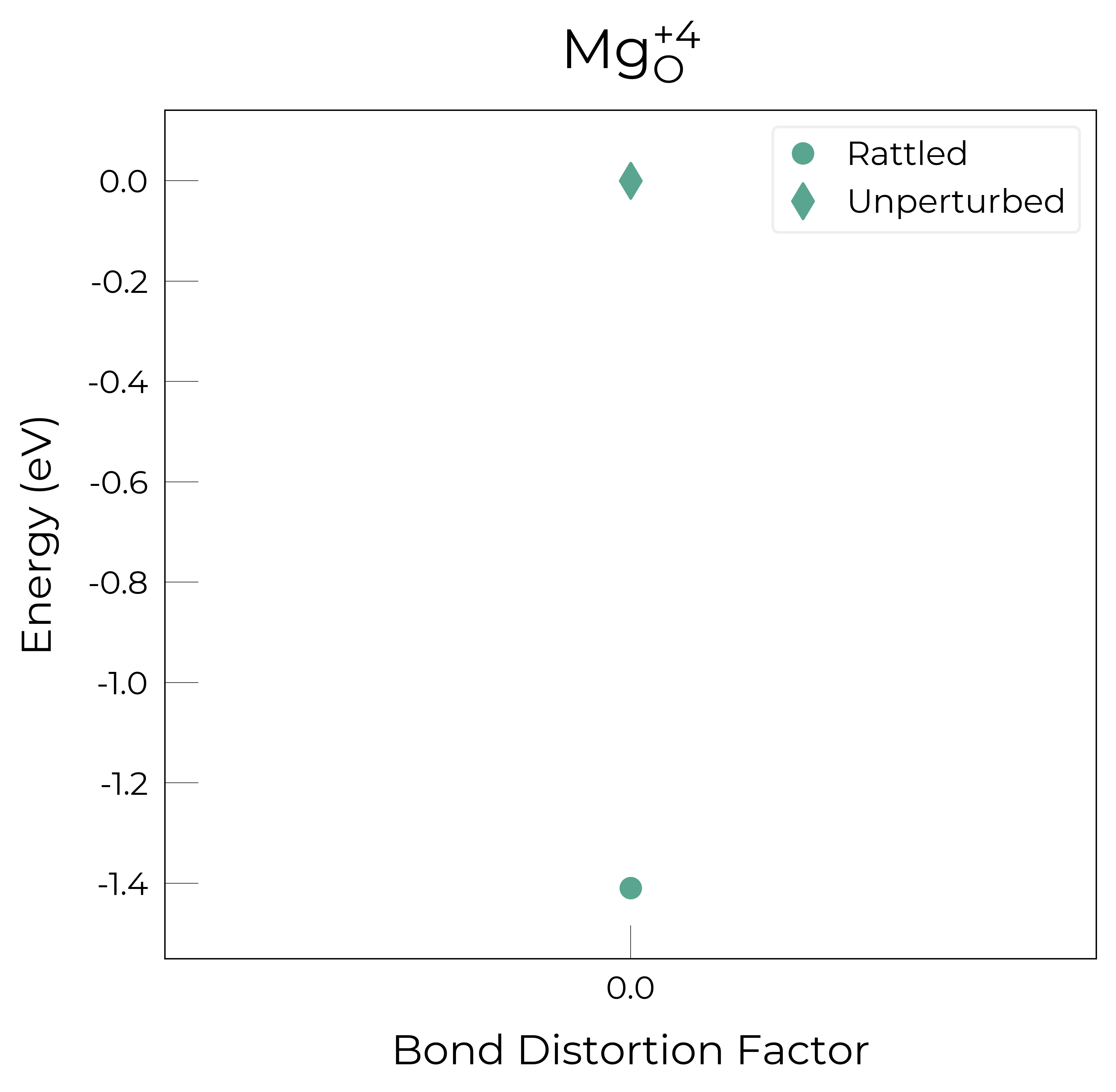
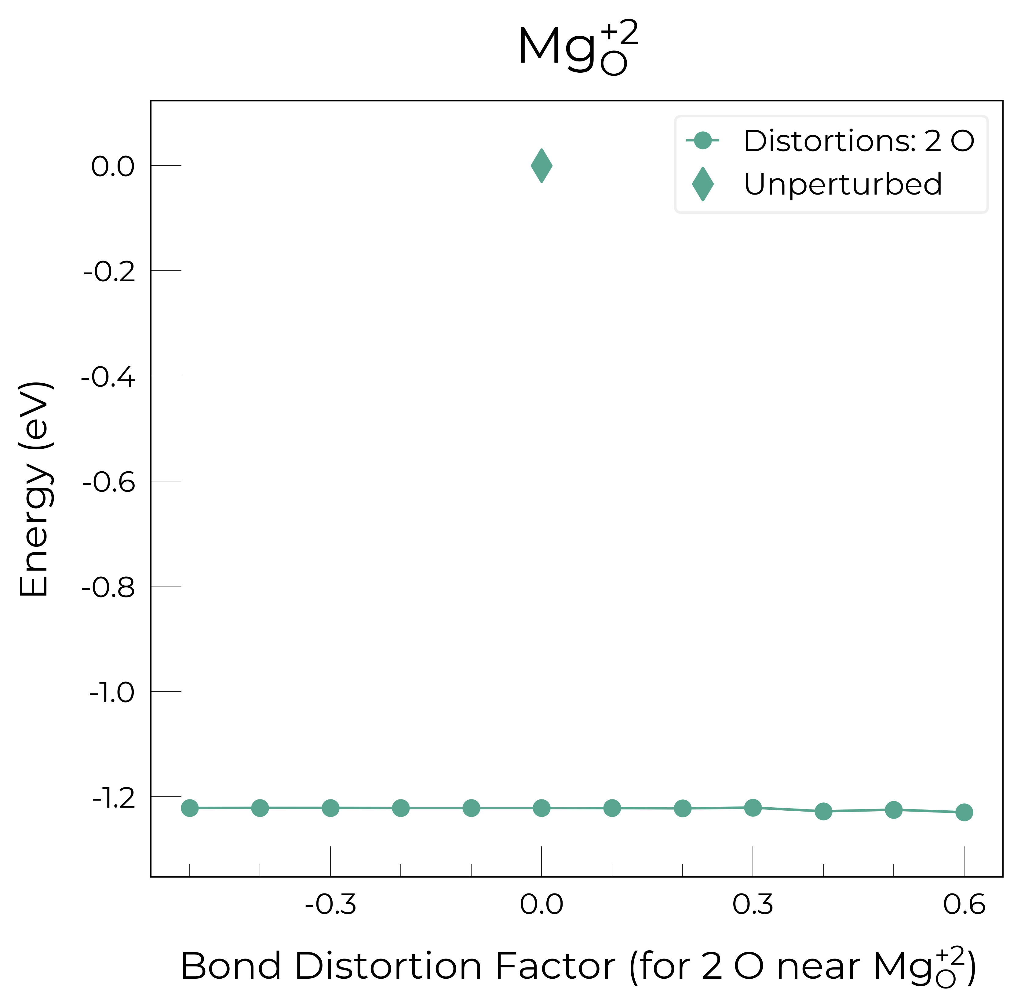
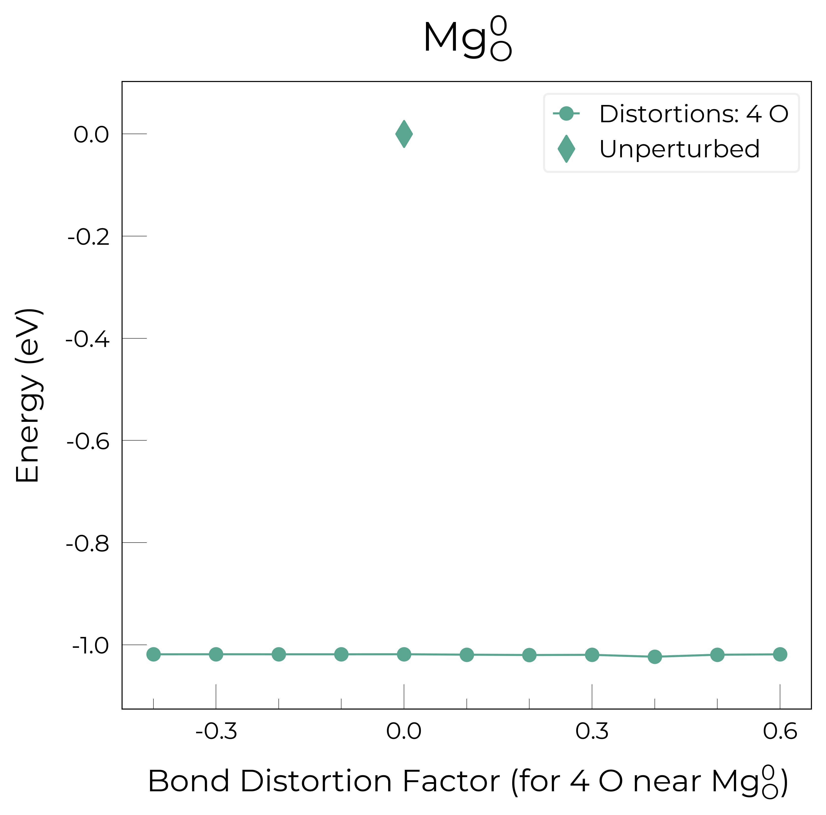
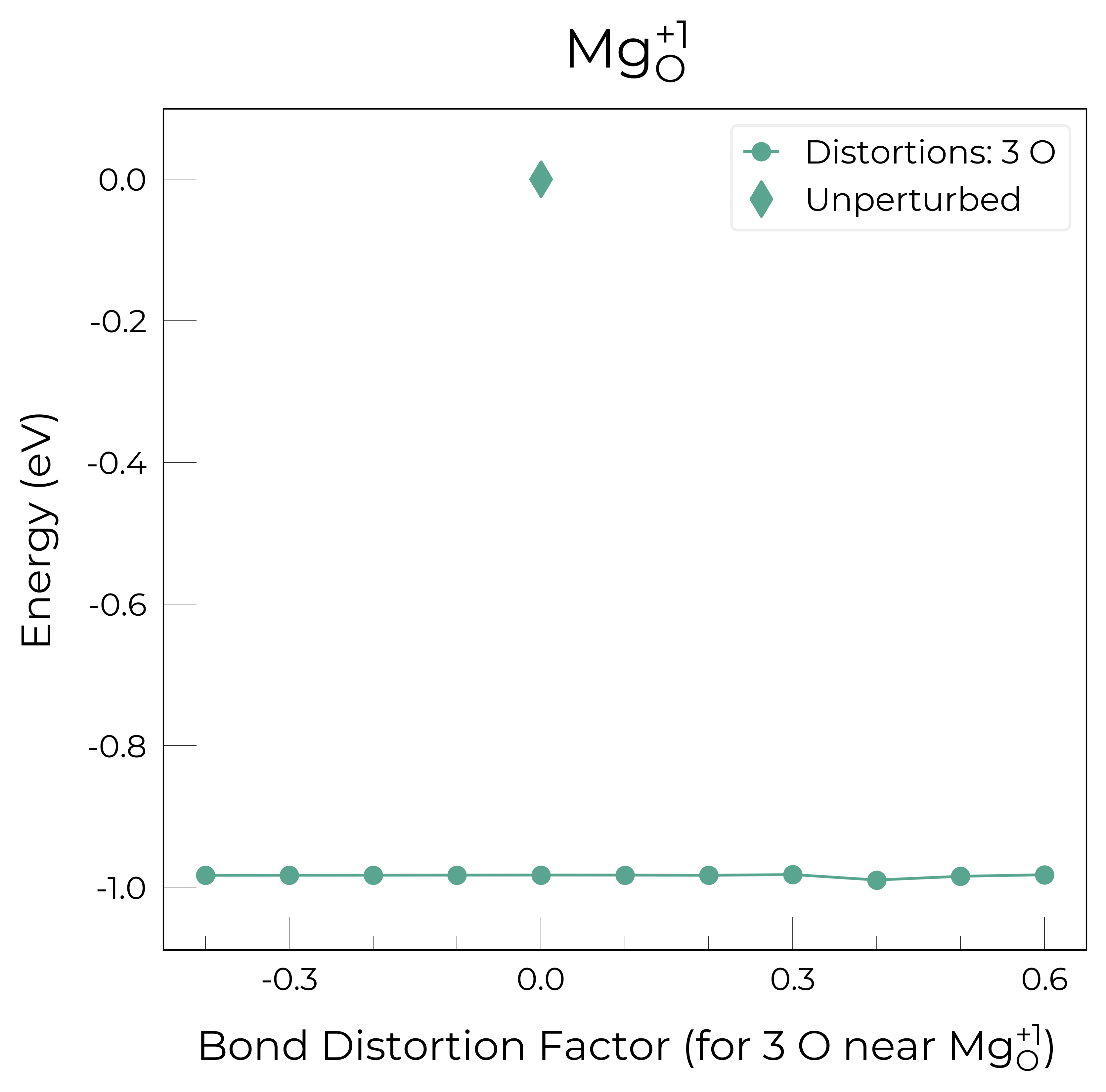
From the plots above, we see that SnB finds energy lowering reconstructions for all charge states of Mg_O. Since the energy lowering is quite high (>0.5 eV), we expect some rebonding to be driving it. We can check this with the SnB function get_homoionic_bonds:
from shakenbreak.analysis import get_energies, get_structures, get_gs_distortion

# Check neutral charge state
energies_mg_0 = get_energies(defect_species="Mg_O_0", output_path="MgO/SnB")
structs_mg_0 = get_structures(defect_species="Mg_O_0", output_path="MgO/SnB")
energy_diff, gs_distortion = get_gs_distortion(energies_mg_0)
s_gs = structs_mg_0[gs_distortion]
s_unperturbed = structs_mg_0["Unperturbed"]
Mg_O_0: Energy difference between minimum, found with 0.4 bond distortion, and unperturbed: -1.02 eV.
The initial ideal structure of the Mg antisite involves a Mg atom surrounded by 6 other Mg. We can check the bond lengths of these bonds in the Unperturbed structure and in the ground state:
from shakenbreak.analysis import get_homoionic_bonds

print("Unperturbed structure:")
unperturbed_bonds = get_homoionic_bonds(
    structure=s_unperturbed,
    elements="Mg",
    radius=2.5,
)
print(f"Ground state structure:")
gs_bonds = get_homoionic_bonds(
    structure=s_gs,
    elements="Mg",
    radius=2.5,
)
Unperturbed structure:
Mg(46): {'Mg(108)': '2.39 A'}

Mg(51): {'Mg(108)': '2.39 A'}

Mg(52): {'Mg(108)': '2.39 A'}

Mg(72): {'Mg(108)': '2.39 A'}

Mg(73): {'Mg(108)': '2.39 A'}

Mg(78): {'Mg(108)': '2.39 A'}

Ground state structure:
Mg(72): {'Mg(108)': '2.24 A'}

Mg(73): {'Mg(108)': '2.24 A'}

Mg(78): {'Mg(108)': '2.24 A'}
So the reconstruction involves replacing 6 Mg-Mg bonds of 2.39 Å by 3 shorter (2.24 Å) and 3 longer bonds. We can visualise the structures with CrystalMaker or Vesta to see the reconstruction:
Unperturbed:

Ground state:

where Mg is shown in yellow, O in red and the Mg antisite is shown in a different pattern.
This distortion likely lowers the electrostatic energy. We can quickly check this by calculating the Madelung energy with pymatgen – as in this study on split vacancies:
# calculate Madelung energy with pymatgen
from pymatgen.core.energy_models import EwaldElectrostaticModel

ewald =  EwaldElectrostaticModel()
# Add oxidation states to structure
s_gs.add_oxidation_state_by_element({"Mg": 2, "O": -2})
s_unperturbed.add_oxidation_state_by_element({"Mg": 2, "O": -2})
ewald_E_gs = ewald.get_energy(s_gs)
ewald_E_unperturbed = ewald.get_energy(s_unperturbed)
print(f"Madelung energy of ground state structure: {ewald_E_gs:.1f} eV")
print(f"Madelung energy of unperturbed structure: {ewald_E_unperturbed:.1f} eV")
print(f"Unscreened electrostatic energy difference (GS - Unperturbed): {ewald_E_gs - ewald_E_unperturbed:.1f} eV")
Madelung energy of ground state structure: -5156.2 eV
Madelung energy of unperturbed structure: -5140.7 eV
Unscreened electrostatic energy difference (GS - Unperturbed): -15.6 eV
Indeed, the ground state structure has a significantly lower Ewald or electrostatic energy. We expect similar driving factors for the other charge states, but you can check them with a similar analysis.
Other functions that may be SnB useful for this analysis are compare_structures(), analyse_structure() and get_site_magnetization() from shakenbreak.analysis; see the distortion analysis section of the SnB Python API tutorial for more.
Below we show the ground state structures for the other charge states:
+1:

+2:

+3:

+4:

For these example results, we find energy lowering distortions for all charge states of MgO. We should re-test these distorted structures for the other charge states where these distortions were not found, in case they also give lower energies.
The get_energy_lowering_distortions() function above automatically performs structure comparisons to determine which distortions should be tested in other charge states of the same defect, and which have already been found (see docstring for more details).
# generates the new distorted structures and VASP inputs, to do our quick 2nd round of structure testing:
energy_lowering_distortions.write_retest_inputs(low_energy_defects, output_path="MgO/SnB")
Writing low-energy distorted structure to MgO/SnB/Mg_O_+4/Bond_Distortion_60.0%_from_+3
Writing low-energy distorted structure to MgO/SnB/Mg_O_0/Rattled_from_+4
Writing low-energy distorted structure to MgO/SnB/Mg_O_+1/Rattled_from_+4
Writing low-energy distorted structure to MgO/SnB/Mg_O_+2/Rattled_from_+4
Writing low-energy distorted structure to MgO/SnB/Mg_O_+3/Rattled_from_+4
Again we run the calculations on the HPCs, then parse and plot the results either using the SnB CLI
functions, or through the python API as exemplified here.
!cp -r MgO/SnB/Pre_Calculated_Results_Regenerate/* MgO/SnB/  # add our pre-calculated results for this step
# skip this if you have run the calculations yourself!
from shakenbreak import energy_lowering_distortions

# re-parse with the same `get_energy_lowering_distortions()` function from before:
defect_charges_dict = energy_lowering_distortions.read_defects_directories(output_path="MgO/SnB")
low_energy_defects = energy_lowering_distortions.get_energy_lowering_distortions(defect_charges_dict, output_path="MgO/SnB")
Mg_O
Mg_O_+3: Energy difference between minimum, found with 0.6 bond distortion, and unperturbed: -1.41 eV.
Energy lowering distortion found for Mg_O with charge +3. Adding to low_energy_defects dictionary.
Mg_O_+4: Energy difference between minimum, found with Rattled bond distortion, and unperturbed: -1.41 eV.
New (according to structure matching) low-energy distorted structure found for Mg_O_+4, adding to low_energy_defects['Mg_O'] list.
Mg_O_+2: Energy difference between minimum, found with 0.6 bond distortion, and unperturbed: -1.23 eV.
Low-energy distorted structure for Mg_O_+2 already found with charge states ['+3'], storing together.
Mg_O_0: Energy difference between minimum, found with 0.4 bond distortion, and unperturbed: -1.02 eV.
Low-energy distorted structure for Mg_O_0 already found with charge states ['+3', '+2'], storing together.
Mg_O_+1: Energy difference between minimum, found with 0.4 bond distortion, and unperturbed: -0.99 eV.
Low-energy distorted structure for Mg_O_+1 already found with charge states ['+3', '+2', '0'], storing together.

Comparing and pruning defect structures across charge states...
Ground-state structure found for Mg_O with charges [3, 2, 0, 1] has also been found for charge state +4 (according to structure matching). Adding this charge to the corresponding entry in low_energy_defects[Mg_O].
Ground-state structure found for Mg_O with charges [4] has also been found for charge state +3 (according to structure matching). Adding this charge to the corresponding entry in low_energy_defects[Mg_O].
from shakenbreak import plotting

figs = plotting.plot_all_defects(defect_charges_dict, output_path="./MgO/SnB")
# set add_colorbar=True for more info in plot
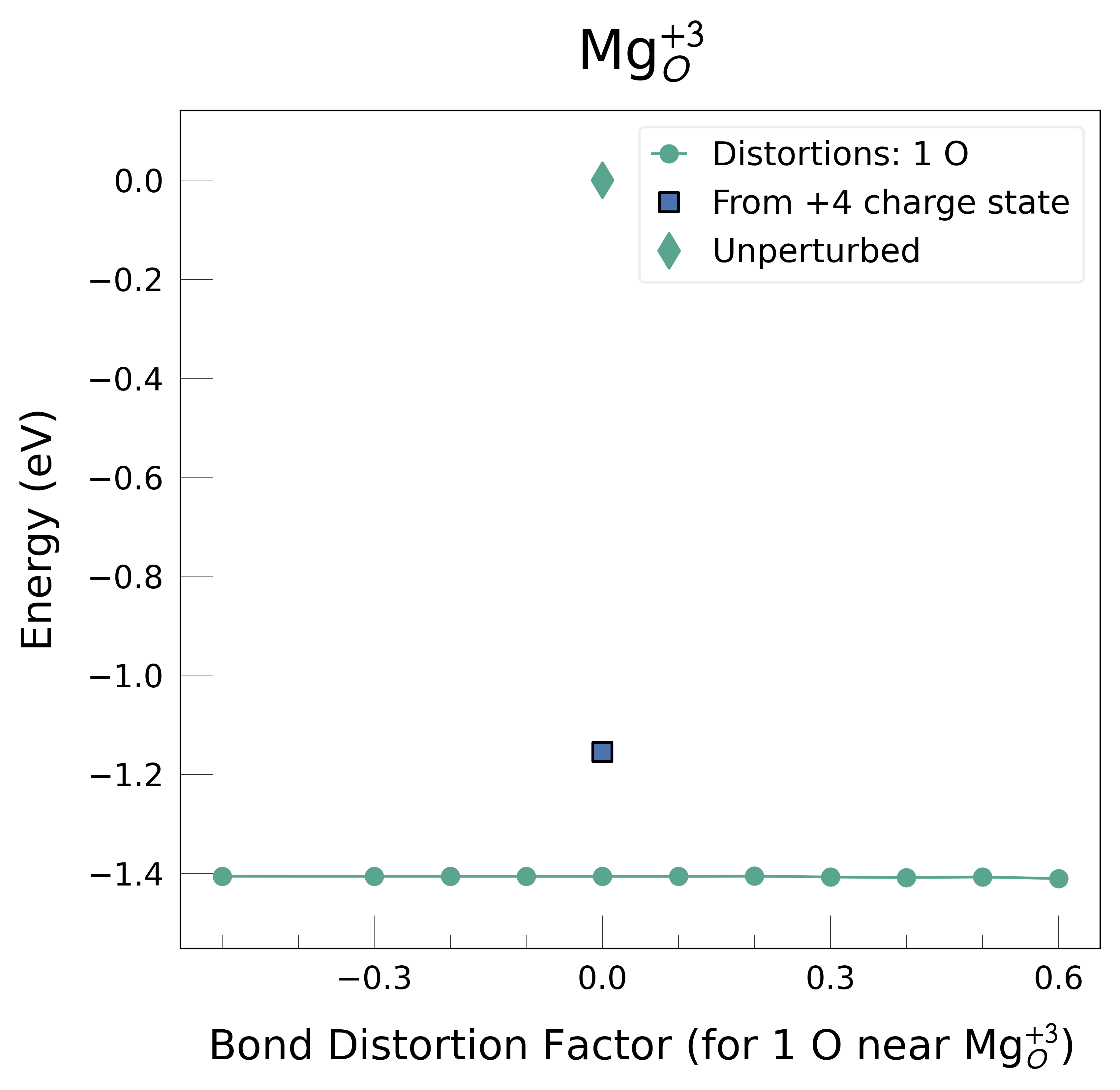
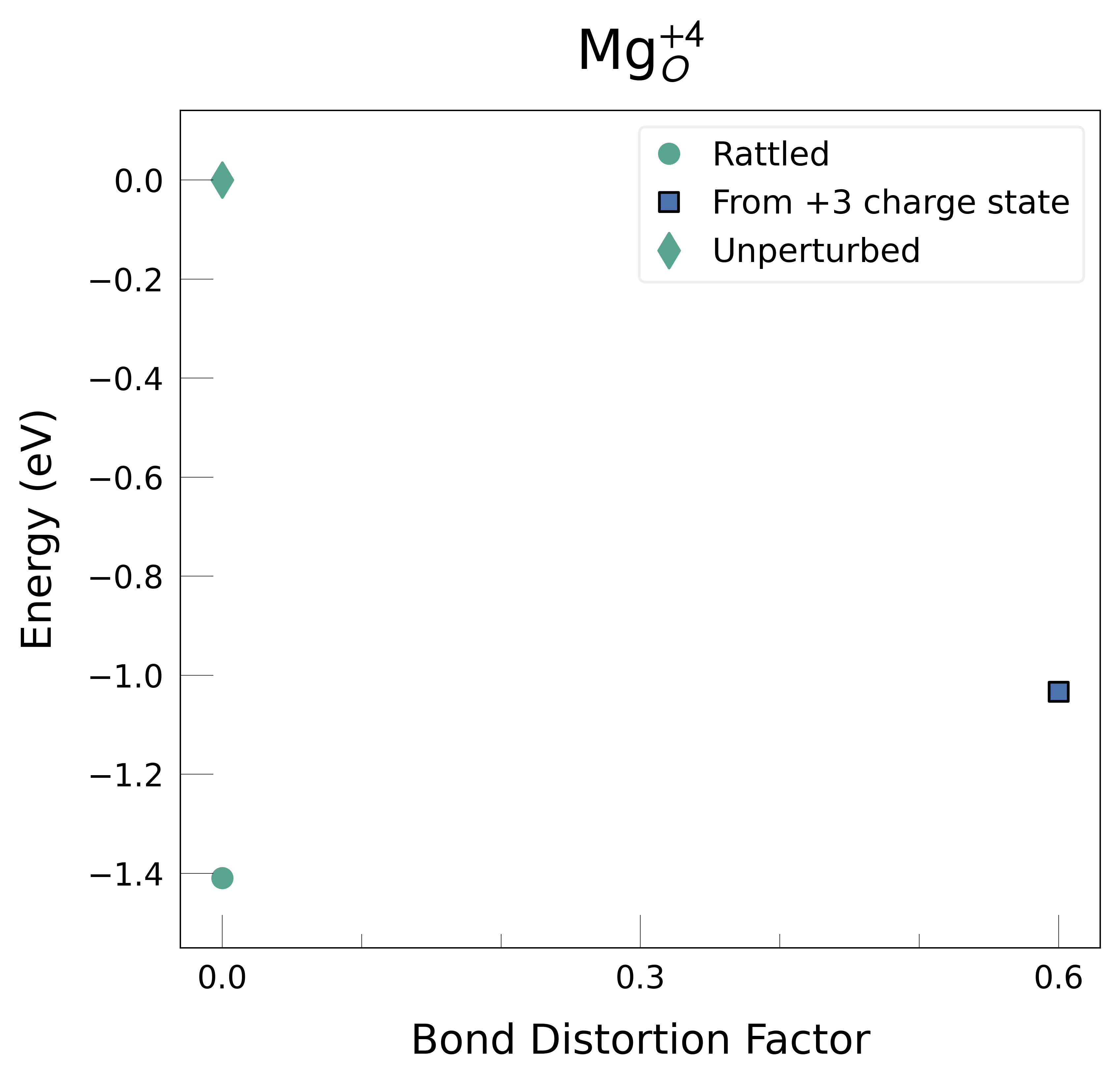
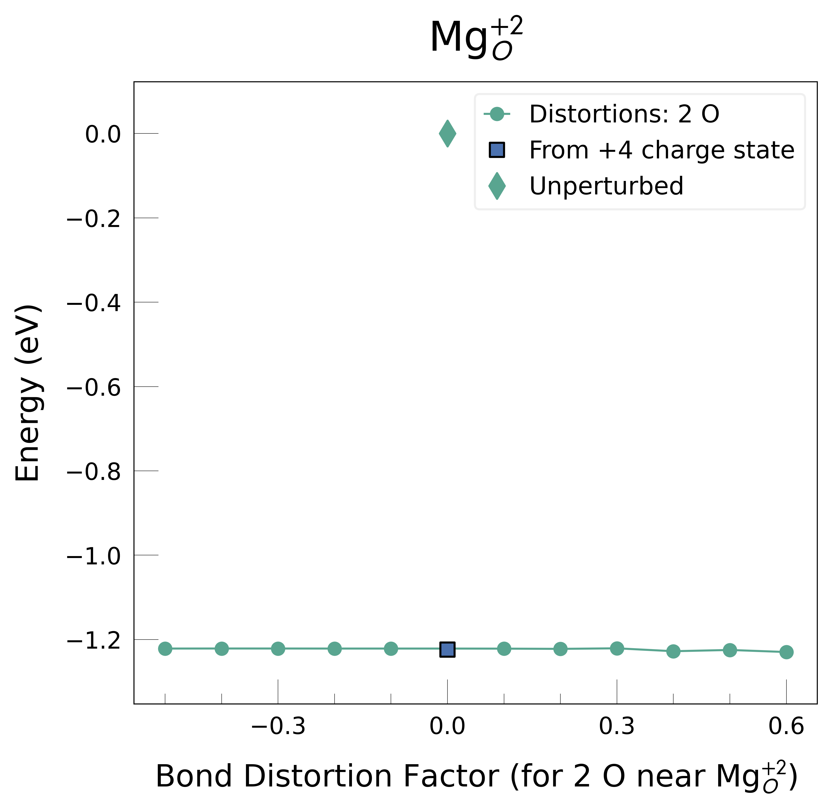
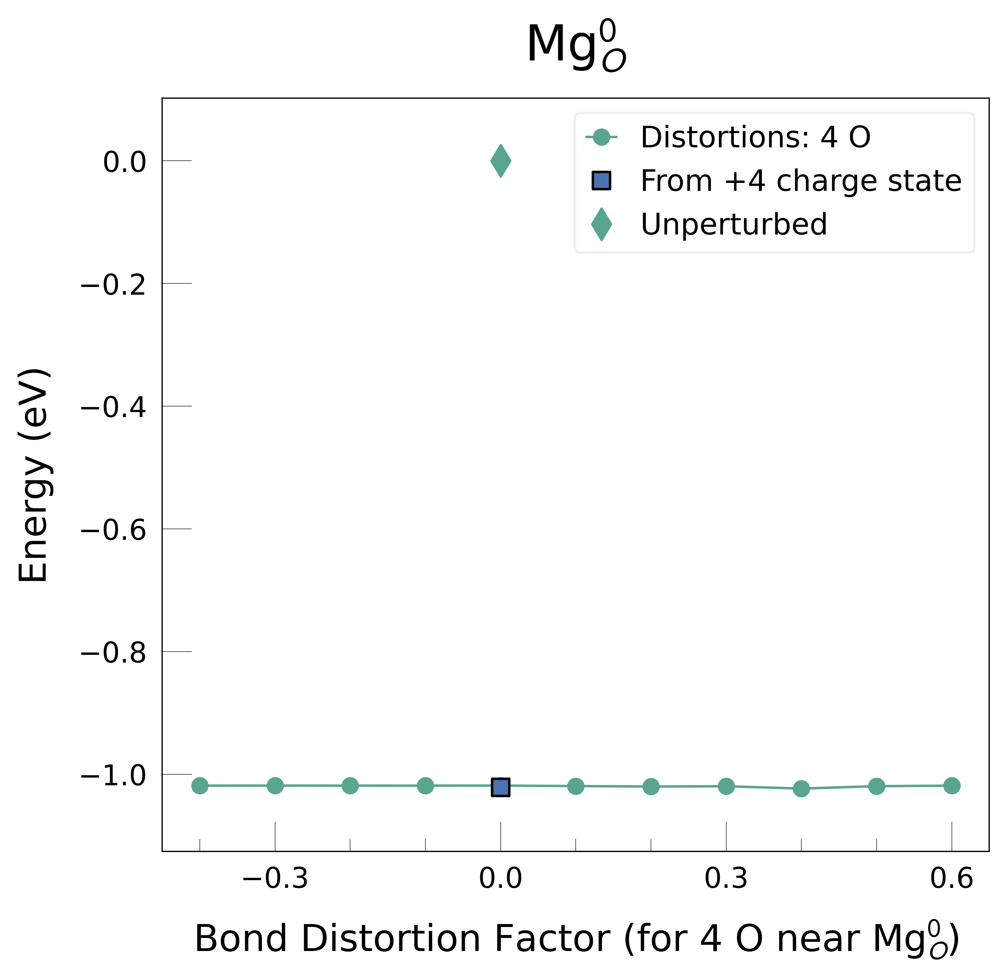
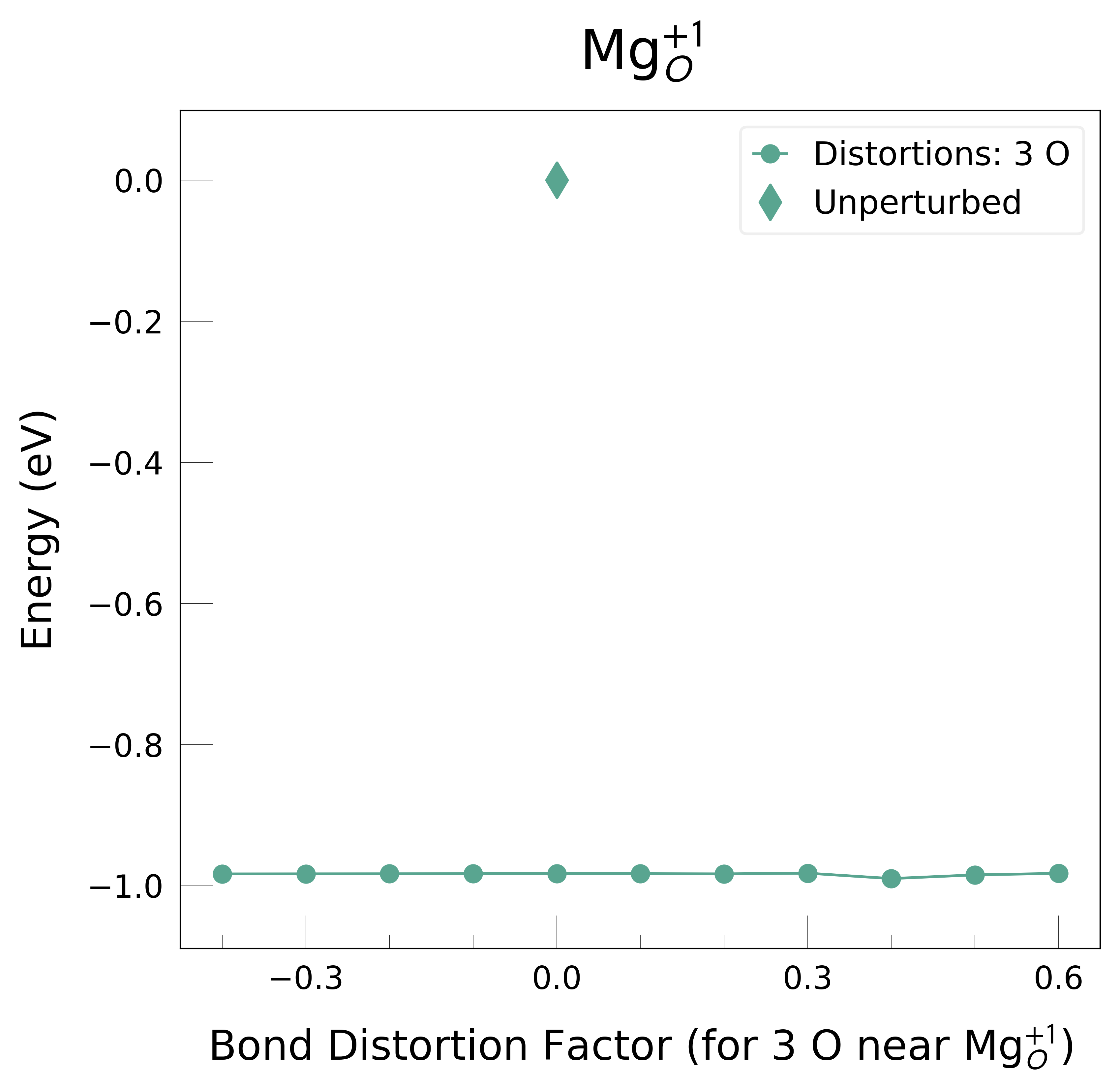
We now continue our defect calculations using the ground-state CONTCARs we’ve obtained for each
defect, with our fully-converged INCAR and KPOINTS settings (via the doped vasp.DefectsSet
class below, to get our final defect formation energies (confident that we’ve identified the ground-state
defect structure!)). The energy_lowering_distortions.write_groundstate_structure() function automatically writes these lowest-energy structures to our defect folders:
energy_lowering_distortions.write_groundstate_structure(output_path="MgO/SnB")
Tip
Usually we would use something like write_groundstate_structure(groundstate_folder="vasp_std", groundstate_filename="POSCAR") (or snb-groundstate -d vasp_std ... on the CLI) as shown in the main doped generation tutorial, which saves the ground-state POSCARs directly to the vasp_std defect subfolders to be used with our later calculations with doped.
However here because we have separated our SnB calculations and doped defect calculations to different folders, we just use the default behaviour (which saves the ground-state structures to groundstate_POSCAR in each defect directory) and will later copy over these POSCAR files.
5. Prepare VASP calculation files with doped
We can estimate the kpoint grid needed for the supercell by calculating the ratio of the supercell lattice parameters to the primitive lattice parameters. For this, we load the DefectGenerator object that we saved earlier:
from doped.generation import DefectsGenerator

defect_gen = DefectsGenerator.from_json("MgO/defect_gen.json.gz")
from pymatgen.core.structure import Structure
import numpy as np

prim_struc = Structure.from_file("MgO/Bulk_relax/CONTCAR")
supercell = defect_gen.bulk_supercell
converged_kgrid = (7, 7, 7)

ratio = np.array(supercell.lattice.abc) / np.array(prim_struc.lattice.abc)
print(f"Ratio of supercell lattice to primitive lattice: {ratio}")
kgrid = tuple(np.array(converged_kgrid) / ratio) # Divide by supercell expansion to get kgrid for supercell
print(f"Kgrid for supercell:", kgrid)
# Round kgrid to next highest integer
print(f"Rounded kgrid for supercell:", [int(np.ceil(k)) for k in kgrid])
Ratio of supercell lattice to primitive lattice: [4.24264069 4.24264069 4.24264069]
Kgrid for supercell: (np.float64(1.6499158228173274), np.float64(1.6499158228173274), np.float64(1.6499158228173274))
Rounded kgrid for supercell: [2, 2, 2]
To generate our VASP input files for the defect calculations, we can use the DefectsSet class in the
vasp module of doped:
from doped.vasp import DefectsSet  # append "?" to function/class to see the help docstrings:
DefectsSet?
Init signature:
DefectsSet(
    defect_entries: doped.generation.DefectsGenerator | dict[str, doped.core.DefectEntry] | list[doped.core.DefectEntry] | doped.core.DefectEntry,
    soc: bool | None = None,
    user_incar_settings: dict | None = None,
    user_kpoints_settings: dict | pymatgen.io.vasp.inputs.Kpoints | None = None,
    user_potcar_functional: str = 'PBE',
    user_potcar_settings: dict | None = None,
    **kwargs,
)
Docstring:
Class for generating input files for ``VASP`` defect calculations for a set
of ``doped``/``pymatgen`` |DefectEntry| objects.
Init docstring:
Creates a dictionary of: ``{defect name: DefectRelaxSet}``.

``DefectRelaxSet`` has the attributes:

- ``DefectRelaxSet.vasp_gam``:
    ``DefectDictSet`` for Gamma-point only relaxation. Usually not
    needed if structure searching (e.g. |ShakeNBreak|) has been
    performed (recommended), unless only Γ-point `k`-point sampling is
    required (converged) for your system, and no ``vasp_std``
    calculations with multiple `k`-points are required (determined from
    kpoint settings).
- ``DefectRelaxSet.vasp_nkred_std``:
    ``DefectDictSet`` for relaxation with a kpoint mesh and using
    ``NKRED``. Not generated for GGA calculations (if ``LHFCALC`` is
    set to ``False`` in ``user_incar_settings``) or if only Gamma
    `k`-point sampling is required.
- ``DefectRelaxSet.vasp_std``:
    ``DefectDictSet`` for relaxation with a kpoint mesh, not using
    ``NKRED``. Not generated if only Gamma kpoint sampling is required.
- ``DefectRelaxSet.vasp_ncl``:
    ``DefectDictSet`` for single-point (static) energy calculation with
    SOC included. Generated if ``soc=True``. If ``soc`` is not set,
    then by default is only generated when the max atomic number (Z)
    over all defect supercells is >= 31 (i.e. further down the periodic
    table than Zn).

where ``DefectDictSet`` is an extension of ``pymatgen``'s
``VaspInputSet`` class for defect calculations, with ``incar``,
``poscar``, ``kpoints`` and ``potcar`` attributes for the corresponding
VASP defect calculations (see docstring). Also creates the
corresponding ``bulk_vasp_...`` attributes for single-point (static)
energy calculations of the bulk (pristine, defect-free) supercell. This
needs to be calculated once with the same settings as the final defect
calculations, for the later calculation of defect formation energies.

See the ``RelaxSet.yaml`` and ``DefectSet.yaml`` files in the
``doped/VASP_sets`` folder for the default ``INCAR`` settings, and
``PotcarSet.yaml`` for the default ``POTCAR`` settings.

Note that any changes to the default ``INCAR``/``POTCAR`` settings
should be consistent with those used for all defect and competing phase
(chemical potential) calculations -- this will be automatically checked
upon defect & competing phases parsing in ``doped``.

Args:
    defect_entries (|DefectsGenerator|, dict/list of |DefectEntry|\s, or |DefectEntry|):
        Either a |DefectsGenerator| object, or a dictionary/list of
        |DefectEntry|\s, or a single |DefectEntry| object, for
        which to generate VASP input files.
        If a |DefectsGenerator| object or a dictionary (->
        ``{defect name: DefectEntry}``), the defect folder names
        will be set equal to ``defect name``. If a list or single
        |DefectEntry| object is provided, the defect folder names
        will be set equal to ``DefectEntry.name`` if the ``name``
        attribute is set, otherwise generated according to the
        ``doped`` convention (see ``doped.generation``).
        Defect charge states are taken from
        ``DefectEntry.charge_state``.
    soc (bool):
        Whether to generate ``vasp_ncl`` ``DefectDictSet`` attribute
        for spin-orbit coupling single-point (static) energy
        calculations. If not set, then by default is set to ``True`` if
        the max atomic number (Z) over all defect supercells is >= 31
        (i.e. further down the periodic table than Zn).
    user_incar_settings (dict):
        Dictionary of user ``INCAR`` settings (AEXX, NCORE etc.) to
        override default settings. Highly recommended to look at output
        ``INCAR``\s or the ``RelaxSet.yaml`` and ``DefectSet.yaml``
        files in the ``doped/VASP_sets`` folder, to see what the
        default ``INCAR`` settings are. Note that any flags that aren't
        numbers or ``True/False`` need to be input as strings with
        quotation marks (e.g. ``{"ALGO": "All"}``).
        (default: None)
    user_kpoints_settings (dict or Kpoints):
        Dictionary of user ``KPOINTS`` settings (in ``pymatgen``
        ``VaspInputSet`` format) e.g., ``{"reciprocal_density": 123}``,
        or a ``Kpoints`` object, to use for the ``vasp_std``,
        ``vasp_nkred_std`` and ``vasp_ncl`` ``DefectDictSet``\s (Γ-only
        for ``vasp_gam``). Default is Gamma-centred,
        ``reciprocal_density = 100`` [kpoints/Å⁻³].
    user_potcar_functional (str):
        ``POTCAR`` functional to use. Default is "PBE" and if this
        fails, tries "PBE_52", then "PBE_54".
    user_potcar_settings (dict):
        Override the default ``POTCAR``\s, e.g. ``{"Li": "Li_sv"}``.
        See ``doped/VASP_sets/PotcarSet.yaml`` for the default
        ``POTCAR`` set.
    **kwargs: Additional kwargs to pass to each ``DefectRelaxSet()``.

Key Attributes:
    defect_sets (dict):
        Dictionary of ``{defect name: DefectRelaxSet}``.
    defect_entries (dict):
        Dictionary of ``{defect name: DefectEntry}`` for the input
        defect species, for which to generate ``VASP`` input files.
    bulk_vasp_gam (DefectDictSet):
        ``DefectDictSet`` for a `bulk` Γ-point-only single-point
        (static) supercell calculation. Often not used, as the bulk
        supercell only needs to be calculated once with the same
        settings as the final defect calculations, which may be with
        ``vasp_std`` or ``vasp_ncl``.
    bulk_vasp_nkred_std (DefectDictSet):
        ``DefectDictSet`` for a single-point (static) `bulk`
        ``vasp_std`` supercell calculation (i.e. with a non-Γ-only
        kpoint mesh) and ``NKRED(X,Y,Z)`` ``INCAR`` tag(s) to
        downsample kpoints for the HF exchange part of the hybrid DFT
        calculation. Not generated for GGA calculations (if ``LHFCALC``
        is set to ``False`` in ``user_incar_settings``) or if only
        Gamma kpoint sampling is required.
    bulk_vasp_std (DefectDictSet):
        ``DefectDictSet`` for a single-point (static) `bulk`
        ``vasp_std`` supercell calculation with a non-Γ-only kpoint
        mesh, not using ``NKRED``. Not generated if only Gamma kpoint
        sampling is required.
    bulk_vasp_ncl (DefectDictSet):
        ``DefectDictSet`` for single-point (static) energy calculation
        of the `bulk` supercell with SOC included. Generated if
        ``soc=True``. If ``soc`` is not set, then by default is only
        generated if the max atomic number (Z) over all defect
        supercells is >= 31 (i.e. further down the periodic table than
        Zn).
    bulk_supercell (|Structure|):
        Supercell structure of the bulk (pristine) material.
    json_obj (dict | |DefectsGenerator|):
        Either the |DefectsGenerator| object if input
        ``defect_entries`` is a |DefectsGenerator| object, otherwise
        the ``defect_entries`` dictionary, which will be written to
        file when ``write_files()`` is called, to aid calculation
        provenance.
    json_name (PathLike):
        Name of the ``JSON`` file to save the ``json_obj`` to.

    Input parameters are also set as attributes.
File:           ~/Packages/doped/doped/vasp.py
Type:           type
Subclasses:
from doped.vasp import DefectsSet  # append "?" to function/class to see the help docstrings:
from pymatgen.io.vasp.inputs import Kpoints

defects_set = DefectsSet(
    defect_gen,  # our DefectsGenerator object, can also input individual DefectEntry objects if desired
    user_incar_settings={
        "ENCUT": 450,
        "GGA": "PS",  # Functional (PBEsol for this tutorial)
        "LHFCALC": False, # Disable Hybrid functional
        "NCORE": 8, # Parallelisation, might need updating for your HPC!
    },  # custom INCAR settings, any that aren't numbers or True/False need to be input as strings with quotation marks!
    user_kpoints_settings=Kpoints(kpts=[(2,2,2)]),
)
# We can also customise the POTCAR settings (and others), see the docstrings above for more info
The DefectsSet class prepares a dictionary in the form {defect_species: DefectRelaxSet}, where
DefectRelaxSet has attributes: vasp_nkred_std (if using hybrid DFT; not the case here), vasp_std (if our final k-point sampling is
non-Γ-only with multiple k-points), vasp_ncl (if SOC included; not the case here as Mg/O are not heavy atoms where SOC is relevant, see docstrings for default behaviour)
and/or vasp_gam (if our final k-point sampling is Γ-only).
These attributes are DefectDictSet objects, subclasses of the pymatgen DictSet object, and contain
information about the calculation inputs.
defects_set.defect_sets
{'Mg_O_+4': doped DefectRelaxSet for bulk composition MgO, and defect entry Mg_O_+4. Available attributes:
 {'_vasp_std', 'defect_supercell', 'bulk_vasp_nkred_std', 'bulk_vasp_gam', 'bulk_vasp_std', 'user_potcar_settings', 'bulk_supercell', 'vasp_std', 'vasp_nkred_std', 'charge_state', 'defect_entry', 'user_kpoints_settings', 'vasp_ncl', 'user_incar_settings', '_vasp_nkred_std', 'user_potcar_functional', 'bulk_vasp_ncl', 'soc', 'vasp_gam', 'poscar_comment', 'dict_set_kwargs'}

 Available methods:
 {'load', 'unsafe_hash', 'write_all', 'write_ncl', 'validate_monty_v1', 'validate_monty_v2', 'save', 'as_dict', 'write_std', 'to_json', 'from_dict', 'write_gam', 'write_nkred_std'},
 'Mg_O_+3': doped DefectRelaxSet for bulk composition MgO, and defect entry Mg_O_+3. Available attributes:
 {'_vasp_std', 'defect_supercell', 'bulk_vasp_nkred_std', 'bulk_vasp_gam', 'bulk_vasp_std', 'user_potcar_settings', 'bulk_supercell', 'vasp_std', 'vasp_nkred_std', 'charge_state', 'defect_entry', 'user_kpoints_settings', 'vasp_ncl', 'user_incar_settings', '_vasp_nkred_std', 'user_potcar_functional', 'bulk_vasp_ncl', 'soc', 'vasp_gam', 'poscar_comment', 'dict_set_kwargs'}

 Available methods:
 {'load', 'unsafe_hash', 'write_all', 'write_ncl', 'validate_monty_v1', 'validate_monty_v2', 'save', 'as_dict', 'write_std', 'to_json', 'from_dict', 'write_gam', 'write_nkred_std'},
 'Mg_O_+2': doped DefectRelaxSet for bulk composition MgO, and defect entry Mg_O_+2. Available attributes:
 {'_vasp_std', 'defect_supercell', 'bulk_vasp_nkred_std', 'bulk_vasp_gam', 'bulk_vasp_std', 'user_potcar_settings', 'bulk_supercell', 'vasp_std', 'vasp_nkred_std', 'charge_state', 'defect_entry', 'user_kpoints_settings', 'vasp_ncl', 'user_incar_settings', '_vasp_nkred_std', 'user_potcar_functional', 'bulk_vasp_ncl', 'soc', 'vasp_gam', 'poscar_comment', 'dict_set_kwargs'}

 Available methods:
 {'load', 'unsafe_hash', 'write_all', 'write_ncl', 'validate_monty_v1', 'validate_monty_v2', 'save', 'as_dict', 'write_std', 'to_json', 'from_dict', 'write_gam', 'write_nkred_std'},
 'Mg_O_+1': doped DefectRelaxSet for bulk composition MgO, and defect entry Mg_O_+1. Available attributes:
 {'_vasp_std', 'defect_supercell', 'bulk_vasp_nkred_std', 'bulk_vasp_gam', 'bulk_vasp_std', 'user_potcar_settings', 'bulk_supercell', 'vasp_std', 'vasp_nkred_std', 'charge_state', 'defect_entry', 'user_kpoints_settings', 'vasp_ncl', 'user_incar_settings', '_vasp_nkred_std', 'user_potcar_functional', 'bulk_vasp_ncl', 'soc', 'vasp_gam', 'poscar_comment', 'dict_set_kwargs'}

 Available methods:
 {'load', 'unsafe_hash', 'write_all', 'write_ncl', 'validate_monty_v1', 'validate_monty_v2', 'save', 'as_dict', 'write_std', 'to_json', 'from_dict', 'write_gam', 'write_nkred_std'},
 'Mg_O_0': doped DefectRelaxSet for bulk composition MgO, and defect entry Mg_O_0. Available attributes:
 {'_vasp_std', 'defect_supercell', 'bulk_vasp_nkred_std', 'bulk_vasp_gam', 'bulk_vasp_std', 'user_potcar_settings', 'bulk_supercell', 'vasp_std', 'vasp_nkred_std', 'charge_state', 'defect_entry', 'user_kpoints_settings', 'vasp_ncl', 'user_incar_settings', '_vasp_nkred_std', 'user_potcar_functional', 'bulk_vasp_ncl', 'soc', 'vasp_gam', 'poscar_comment', 'dict_set_kwargs'}

 Available methods:
 {'load', 'unsafe_hash', 'write_all', 'write_ncl', 'validate_monty_v1', 'validate_monty_v2', 'save', 'as_dict', 'write_std', 'to_json', 'from_dict', 'write_gam', 'write_nkred_std'}}
# for example, let's look at the generated inputs for a `vasp_std` calculation for Mg_O_0:
print(f"INCAR:\n{defects_set.defect_sets['Mg_O_0'].vasp_std.incar}")
print(f"KPOINTS:\n{defects_set.defect_sets['Mg_O_0'].vasp_std.kpoints}")
print(f"POTCAR (symbols):\n{defects_set.defect_sets['Mg_O_0'].vasp_std.potcar_symbols}")
INCAR:
# MAY WANT TO CHANGE NCORE, KPAR, AEXX, ENCUT, IBRION, LREAL, NUPDOWN, ISPIN, MAGMOM = Typical variable parameters
ALGO = Normal  # change to all if zhegv, fexcp/f or zbrent errors encountered, or poor electronic convergence
EDIFF = 1e-05
EDIFFG = -0.01
ENCUT = 450.0
GGA = Ps
IBRION = 2
ICHARG = 1
ICORELEVEL = 0
ISEARCH = 1
ISIF = 2
ISMEAR = 0
ISPIN = 2
ISYM = 0
KPAR = 4
LASPH = True
LHFCALC = False
LORBIT = 11
LREAL = Auto
LVHAR = True
NCORE = 8
NEDOS = 3000
NSW = 200
NUPDOWN = 0.0
PREC = Accurate
SIGMA = 0.05

KPOINTS:
KPOINTS from doped
0
Gamma
2 2 2

POTCAR (symbols):
['Mg', 'O']
Tip
The use of (subclasses of) pymatgen DictSet objects here allows these functions to be readily used with high-throughput frameworks such as atomate(2) or AiiDA.
We can then write these files to disk with the write_files() method:
defects_set.write_files?
Signature:
defects_set.write_files(
    output_path: str | pathlib._local.Path = '.',
    poscar: bool = False,
    rattle: bool = True,
    vasp_gam: bool | None = None,
    bulk: bool | str = True,
    processes: int | None = None,
    **kwargs,
)
Docstring:
Write VASP input files to folders for all defects in
``self.defect_entries``. Folder names are set to the key of the
DefectRelaxSet in ``self.defect_sets`` (same as self.defect_entries
keys, see |DefectsSet| docstring).

For each defect folder, the following subfolders are generated:

- ``vasp_nkred_std``:
    Defect relaxation with a kpoint mesh and using ``NKRED``. Not
    generated for GGA calculations (if ``LHFCALC`` is set to ``False``
    in ``user_incar_settings``) or if only Γ-point sampling required.
- ``vasp_std``:
    Defect relaxation with a kpoint mesh, not using ``NKRED``. Not
    generated if only Γ-point sampling required.
- ``vasp_ncl``:
    Singlepoint (static) energy calculation with SOC included.
    Generated if ``soc=True``. If ``soc`` is not set, then by default
    is only generated if the max atomic number (Z) over all defect
    supercells is >= 31 (i.e. further down the periodic table than Zn).

If ``vasp_gam=True`` (not recommended) or ``self.vasp_std = None``
(i.e. Γ-only `k`-point sampling converged for the kpoints settings
used), then also outputs:

- ``vasp_gam``:
    Γ-point only defect relaxation. Usually not needed if structure
    searching has been performed (e.g. with |ShakeNBreak|)
    (recommended).

By default, does not generate a ``vasp_gam`` folder unless
``DefectRelaxSet.vasp_std`` is ``None`` (i.e. only Γ-point sampling
required for this system), as ``vasp_gam`` calculations should be
performed with defect structure-searching (e.g. with |ShakeNBreak|)
and initial relaxations. If ``vasp_gam`` files are desired, set
``vasp_gam=True``.

By default, ``POSCAR`` files are not generated for the
``vasp_(nkred_)std`` (and ``vasp_ncl`` if ``self.soc`` is ``True``)
folders, as these should be taken from structure-searching calculations
(e.g. ``snb-groundstate -d vasp_nkred_std``) or, if not following the
recommended structure-searching workflow, from the ``CONTCAR``\s of
``vasp_gam`` calculations. If including SOC effects (i.e.
``self.soc = True``), then the ``vasp_std`` ``CONTCAR``\s should be
used as the ``vasp_ncl`` ``POSCAR``\s. If ``POSCAR`` files are desired
for the ``vasp_(nkred_)std`` (and ``vasp_ncl``) folders, set
``poscar=True``.

Input files for the single-point (static) bulk supercell reference
calculation are also written to ``"{formula}_bulk/{subfolder}"`` if
``bulk`` is ``True`` (default), where ``subfolder`` corresponds to the
final (highest accuracy) VASP calculation in the workflow (i.e.
``vasp_ncl`` if ``self.soc=True``, otherwise ``vasp_std`` or
``vasp_gam`` if only Γ-point reciprocal space sampling is required). If
``bulk = "all"``, then the input files for all VASP calculations
(gam/std/ncl) are written to the bulk supercell folder, or if
``bulk = False``, then no bulk folder is created.

The |DefectEntry| objects are also written to ``json.gz`` files in
the defect folders, as well as ``self.defect_entries``
(``self.json_obj``) in the top folder, to aid calculation provenance
-- these can be reloaded directly with ``loadfn()`` from
``monty.serialization``, or individually with
``DefectEntry.from_json()``.

See the ``RelaxSet.yaml`` and ``DefectSet.yaml`` files in the
``doped/VASP_sets`` folder for the default ``INCAR`` and ``KPOINT``
settings, and ``PotcarSet.yaml`` for the default ``POTCAR`` settings.
**These are reasonable defaults that `roughly` match the typical values
needed for accurate defect calculations, but usually will need to be
modified for your specific system, such as converged ENCUT and KPOINTS,
and NCORE / KPAR matching your HPC setup.**

Note that any changes to the default ``INCAR``/``POTCAR`` settings
should be consistent with those used for all defect and competing phase
(chemical potential) calculations -- this will be automatically checked
upon defect & competing phases parsing in ``doped``.

Args:
    output_path (PathLike):
        Folder in which to create the VASP defect calculation folders.
        Default is the current directory ("."). Output folder structure
        is ``<output_path>/<defect name>/<subfolder>`` where
        ``defect name`` is the key of the DefectRelaxSet in
        ``self.defect_sets`` (same as ``self.defect_entries`` keys, see
        |DefectsSet| docstring) and ``subfolder`` is the name of the
        corresponding VASP program to run (e.g. ``vasp_std``).
    poscar (bool):
        If ``True``, writes the defect ``POSCAR`` to the generated
        folders as well. Typically not recommended, as the recommended
        workflow is to initially perform ``vasp_gam`` ground-state
        structure searching using |ShakeNBreak|
        (https://shakenbreak.readthedocs.io) or another approach, then
        continue the ``vasp(_nkred)_std`` relaxations from the
        ground-state structures (e.g. using ``-d vasp_nkred_std`` with
        ``snb-groundstate`` (CLI) or
        ``groundstate_folder="vasp_nkred_std"`` with
        ``write_groundstate_structure`` (Python API)), first with
        ``NKRED`` if using hybrid DFT, then without ``NKRED``.
        (default: False)
    rattle (bool):
        If writing ``POSCAR``\s, apply random displacements to all
        atomic positions in the structures using the |ShakeNBreak|
        algorithm; i.e. with the displacement distances randomly drawn
        from a Gaussian distribution of standard deviation equal to 10%
        of the bulk nearest neighbour distance and using a Monte Carlo
        algorithm to penalise displacements that bring atoms closer
        than 80% of the bulk nearest neighbour distance.
        ``stdev`` and ``d_min`` can also be given as input kwargs.
        This is intended to be used as a fallback option for breaking
        symmetry to partially aid location of global minimum defect
        geometries, if |ShakeNBreak| structure-searching is being
        skipped. However, rattling still only finds the ground-state
        structure for <~30% of known cases of energy-lowering
        reconstructions relative to an unperturbed defect structure.
        (default: True)
    vasp_gam (bool | None):
        If ``True``, writes the ``vasp_gam`` input files, with defect
        ``POSCAR``\s. Not recommended, as the recommended workflow is
        to initially perform ``vasp_gam`` ground-state structure
        searching (e.g. using |ShakeNBreak|;
        https://shakenbreak.readthedocs.io), then continue the
        ``vasp_std`` relaxations from the ground-state structures.
        Default is ``None``, where ``vasp_gam`` folders are written if
        ``self.vasp_std`` is ``None`` (i.e. only Γ-point reciprocal
        space sampling is required).
    bulk (bool, str):
        If ``True``, the input files for a single-point calculation of
        the bulk supercell are also written to
        ``"{formula}_bulk/{subfolder}"``, where ``subfolder``
        corresponds to the final (highest accuracy) ``VASP``
        calculation in the workflow (i.e. ``vasp_ncl`` if
        ``self.soc=True``, otherwise ``vasp_std`` or ``vasp_gam`` if
        only Γ-point reciprocal space sampling is required). If
        ``bulk = "all"`` then the input files for all ``VASP``
        calculations in the workflow (``vasp_gam``, ``vasp_nkred_std``,
        ``vasp_std``, ``vasp_ncl`` (if applicable)) are written to the
        bulk supercell folder.
        (Default: False)
    processes (int):
        Number of processes to use for ``multiprocessing`` for file
        writing. If ``None`` (default), then is dynamically set to the
        optimal value for the number of folders to write.
        (Default: None)
    **kwargs:
        Keyword arguments to pass to ``DefectDictSet.write_input()``.
File:      ~/Packages/doped/doped/vasp.py
Type:      method
# cannot be run on Colab: (can't automatically write charged defect INCAR/POTCAR as this
# requires POTCARs to be setup with pymatgen; https://doped.readthedocs.io/en/latest/Installation.html)
defects_set.write_files(output_path="./MgO/Defects")
Generating and writing input files: 100%|██████████| 5/5 [00:00<00:00, 28.06it/s]
# # one can write input files (except for POTCAR) on Colab for neutral defects (otherwise
# # POTCAR files needed to specify NELECT (number of electrons) for charged systems):
# defects_set["Mg_O_0"].write_all(defect_dir="./MgO/Defects/Mg_O_0", potcar_spec=True)
Note
The recommended defects workflow is to use the ShakeNBreak approach with the initial generated defect configurations, which allows us to identify the ground-state structures and also accelerates the defect calculations by performing the initial fast vasp_gam relaxations, which ‘pre-converge’ our structures by bringing us very close to the final converged relaxed structure, much quicker (10-100x) than if we performed the fully-converged vasp_std relaxations from the beginning.
As such, DefectsSet.write_files() assumes by default that the defect structures (POSCARs) have
already been generated and pre-relaxed with ShakeNBreak, and that you will then copy in the
ground-state POSCARs (as shown below) to continue with the final defect relaxations in these folders.
If for some reason you are not following this recommended approach, you can either set vasp_gam = True
in write_files() to generate the unperturbed defect structures and input files for vasp_gam
relaxations, or you can use unperturbed_poscar = True to also write the unperturbed defect POSCARs
to the defect folders.
!ls ./MgO/Defects/*Mg_O*/*vasp* # list the generated VASP input files
./MgO/Defects/Mg_O_+1/vasp_std:
INCAR           KPOINTS         Mg_O_+1.json.gz POTCAR

./MgO/Defects/Mg_O_+2/vasp_std:
INCAR           KPOINTS         Mg_O_+2.json.gz POTCAR

./MgO/Defects/Mg_O_+3/vasp_std:
INCAR           KPOINTS         Mg_O_+3.json.gz POTCAR

./MgO/Defects/Mg_O_+4/vasp_std:
INCAR           KPOINTS         Mg_O_+4.json.gz POTCAR

./MgO/Defects/Mg_O_0/vasp_std:
INCAR          KPOINTS        Mg_O_0.json.gz POTCAR
We can see that for each defect species, we have a vasp_std folder
with corresponding VASP input files. This follows our recommended defect workflow
(YouTube, B站),
which is to first perform defect structure-searching with ShakeNBreak using vasp_gam, then copy in the
pre-relaxed ground-state POSCARs to continue the final fully-converged defect relaxations with
vasp_std/vasp_gam (depending on the converged k-point set). Note that if you were using a hybrid
functional, there will be an extra step before the final vasp_std where we would use NKRED to reduce
the cost of hybrid DFT calculations (typically good accuracy for forces)(-> vasp_nkred_std input files).
Then we would continue the relaxation without NKRED (-> vasp_std folder).
Additionally, if SOC is important for your system (typically with elements in period 5 and below),
we’d do a final SOC singlepoint calculation with vasp_ncl.
Copy over our ground-state POSCARs (from the MgO/SnB folders) to the defect folders (in MgO/Defects):
import shutil
import os

for defect in os.listdir("./MgO/SnB/"):  # will fail on Colab; files not written for charged defect folders
    # if last character of defect is a number (i.e. charge state)
    if defect[-1].isnumeric():
        shutil.copy(
            os.path.join("./MgO/SnB/", defect, "groundstate_POSCAR"),
            os.path.join("./MgO/Defects/", defect, "vasp_std", "POSCAR")
        )
Note
The NELECT INCAR tag (-> number of electrons, sets the defect charge state in the calculation) is
automatically determined based on the choice of POTCARs. The default in both doped and ShakeNBreak
is to use the MPRelaxSet POTCAR choices, but if
you’re using different ones, make sure to set potcar_settings in the VASP file generation functions,
so that NELECT is then set accordingly. This requires the pymatgen config file $HOME/.pmgrc.yaml
to be properly set up as detailed on the Installation docs page
As well as the INCAR, POTCAR and KPOINTS files for each calculation in the defects workflow, we
also see that a {defect_species}.json file is created by default, which contains the corresponding
DefectEntry python object, which can later be reloaded with DefectEntry.from_json() (useful if we
later want to recheck some of the defect generation info).
The DefectsGenerator object is also saved to JSON by default here, which can be reloaded with
DefectsGenerator.from_json().
A folder with the input files for calculating the reference bulk (pristine, defect-free) supercell is also generated (this calculation is needed to later compute defect formation energies and charge corrections):
!ls MgO/Defects/MgO_bulk/vasp_std # only the final workflow VASP calculation is required for the bulk, see docstrings
INCAR KPOINTS POSCAR POTCAR
6. Chemical Potentials
Here we show a quick guide on how to do this. For a more extensive guide, check this tutorial.
To calculate the limiting chemical potentials of elements in the material (needed for calculating the defect formation energies) we need to consider the energies of all competing phases. doped does this by calling the CompetingPhases class, which then queries Materials Project to obtain all the relevant competing phases to be calculated.
In some cases the Materials Project may not have all known phases in a certain chemical space, so it’s a good idea to cross-check the generated competing phases with the ICSD in case you suspect any are missing.
For this functionality to work correctly, you will need an API key for the Materials Project (as described on the Installation docs page).
from doped.chemical_potentials import CompetingPhases
cp = CompetingPhases(  # SK API key -- replace with yours!
    "MgO", energy_above_hull=0.01, api_key="UsPX9Hwut4drZQXPTxk4CwlCstrAAjDv"
)  # low energy_above_hull for this tutorial example

# if you don't have your MP API key set up in ~/.pmgrc.yaml (see Installation docs),
# you can supply it as a parameter in this function, or set it as an env var with:
# !export MP_API_KEY="your_api_key"
The default thermo type when retrieving entries has been changed from the mixed/corrected PBE GGA and GGA+U hull (`thermo_type = GGA_GGA+U`) to the joint PBE GGA / GGA+U / r2SCAN hull (`thermo_type = GGA_GGA+U_R2SCAN`). To use the older behavior, call `get_entries_in_chemsys` with `additional_criteria = {"thermo_types": ["GGA_GGA+U"]}`
Note
The current algorithm for how doped queries the Materials Project (MP) and determines relevant competing phases to be calculated, is that it first queries the MP for all phases with energies above hull less than energy_above_hull (optional parameter in CompetingPhases()) in eV/atom in the chemical space of the host material. It then determines which of these phases border the host material in the phase diagram (i.e. which are competing phases and thus determine the chemical potentials), as well as which phases would border the host material if their energies were downshifted by energy_above_hull. The latter are included as well, and so energy_above_hull acts as an uncertainty range for the MP-calculated formation energies, which may not be accurate due to functional choice (GGA vs hybrid DFT / GGA+U / RPA etc.), lack of vdW corrections etc.
In this qualitative tutorial, since we’re using GGA, we use a less strict energy_above_hull than the default (0.01 vs 0.1 eV/atom). But in general, it’s recommended to use the default energy_above_hull of 0.1 eV/atom, which is a reasonable value.
cp.entries contains pymatgen ComputedStructureEntry objects for all the relevant competing phases, which includes useful data such as their structures, magnetic moment and (MP-calculated GGA) band gaps.
print(len(cp.entries))
print([entry.name for entry in cp.entries])
5
['MgO', 'Mg', 'O2', 'Mg', 'Mg']
We can plot our phase diagram like this, which can show why certain phases are included as competing phases:
import doped
import matplotlib.pyplot as plt
plt.style.use(f"{doped.__path__[0]}/utils/doped.mplstyle")  # use doped style
from mp_api.client import MPRester
from pymatgen.analysis.phase_diagram import PhaseDiagram, PDPlotter

system = ["Mg", "O"]  # system we want to get phase diagram for
# object for connecting to MP Rest interface, may need to specify API key here
mpr = MPRester(api_key="UsPX9Hwut4drZQXPTxk4CwlCstrAAjDv")  # SK API key -- replace with yours!
entries = mpr.get_entries_in_chemsys(system)  # get all entries in the chemical system
pd = PhaseDiagram(entries)  # create phase diagram object
plotter = PDPlotter(pd, show_unstable=0.01, backend="matplotlib")  # plot phase diagram
plot = plotter.get_plot()
895872525.py:10: MPRestWarning: The default thermo type when retrieving entries has been changed from the mixed/corrected PBE GGA and GGA+U hull (`thermo_type = GGA_GGA+U`) to the joint PBE GGA / GGA+U / r2SCAN hull (`thermo_type = GGA_GGA+U_R2SCAN`). To use the older behavior, call `get_entries_in_chemsys` with `additional_criteria = {"thermo_types": ["GGA_GGA+U"]}`
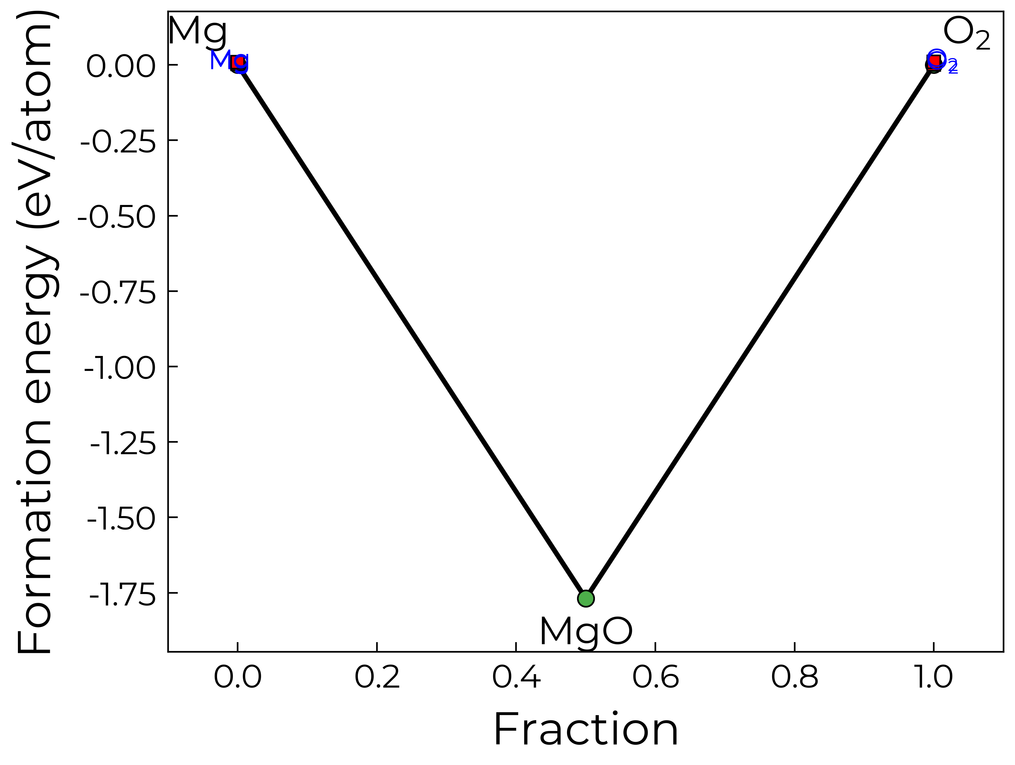
Which shows that there are two low-energy polymorphs of Mg on the MP database.
6.1 Generating input files
We can then set up the competing phase calculations with doped as described below, or use the pymatgen ComputedStructureEntry objects in cp.entries to set these up in your desired format with python / atomate / AiiDA etc.
k-points convergence testing is done at GGA (PBEsol by default) and is set up to account for magnetic moment convergence as well. Here we interface with vaspup2.0 to make it easy to use on the HPCs (with the generate-converge command to run the calculations and data-converge to quickly parse and analyse the results).
You may want to change the default ENCUT (350 eV) or k-point densities that the convergence tests span (5 - 60 kpoints/Å3 for semiconductors & insulators and 40 - 120 kpoints/Å3 for metals in steps of 5 kpoints/Å3). Note that ISMEAR = -5 is used for metals by default (better kpoint convergence for energies but should not be used during metal geometry relaxations) and k-point convergence testing is not required for molecules (Γ-point sampling is sufficient).
Note that doped generates “molecule in a box” structures for the gaseous elemental phases
H2, O2, N2, F2 and Cl2. The molecule is placed in
a slightly-symmetry-broken (to avoid metastable electronic solutions) 30 Å cuboid box, and relaxed with Γ-point-only k-point sampling.
The kpoints convergence calculations are set up with:
6.1.1 Convergence calculations
Prepare input files
# Update some INCAR settings:
# GGA functional to PBEsol
# NCORE to the correct value for our HPC
# And increase NELM from deafult (60) as metals can take longer to converge
cp.convergence_setup(  # now renamed to `write_kpoint_convergence_files`
    # For custom INCAR settings:
    # any flags that aren't numbers or True/False need to be input as strings with quotation marks:
    user_incar_settings={'GGA': "PS", "LHFCALC": False, "AEXX": 0.0, "HFSCREEN": 0.0, "NCORE": 8, "NELM": 120},
    # potcar_spec=True  # uncomment to run on Colab!
)
1782699770.py:5: DeprecationWarning: `CompetingPhases.convergence_setup` is deprecated and will be removed in the next minor release (v4.1); use `CompetingPhases.write_kpoint_convergence_files` instead.
Note that diatomic molecular phases, calculated as molecules-in-a-box (O2 in this case), do not require k-point convergence testing, as Γ-only sampling is sufficient.
{'CompetingPhases/MgO_Fm-3m_EaH_0/kpoint_converge/k4,4,4': doped DopedDictSet with structure composition Mg1 O1. Available attributes:
 {'prev_vasprun', 'auto_metal_kpoints', 'vdw', 'potcar_functional', 'sym_prec', 'structure', 'user_potcar_settings', 'kpoints', 'charge_state', 'validate_magmom', 'incar', 'user_kpoints_settings', 'nelect', 'use_structure_charge', 'prev_incar', 'potcar', 'constrain_total_magmom', 'reduce_structure', 'auto_kpar', 'force_gamma', 'poscar', 'kpoints_updates', 'auto_kspacing', 'sort_structure', 'standardize', 'potcar_symbols', 'incar_updates', 'config_dict', 'user_incar_settings', 'prev_kpoints', 'user_potcar_functional', 'files_to_transfer', 'international_monoclinic', 'auto_ispin', 'prev_outcar', 'auto_ismear', 'bandgap', 'poscar_comment', 'inherit_incar', 'auto_lreal', 'bandgap_tol'}

 Available methods:
 {'load', 'unsafe_hash', 'from_directory', 'get_input_set', 'validate_monty_v1', 'write_input', 'calculate_ng', 'validate_monty_v2', 'as_dict', 'save', 'override_from_prev_calc', 'get_vasp_input', 'estimate_nbands', 'to_json', 'from_dict', 'from_prev_calc'},
 'CompetingPhases/MgO_Fm-3m_EaH_0/kpoint_converge/k5,5,5': doped DopedDictSet with structure composition Mg1 O1. Available attributes:
 {'prev_vasprun', 'auto_metal_kpoints', 'vdw', 'potcar_functional', 'sym_prec', 'structure', 'user_potcar_settings', 'kpoints', 'charge_state', 'validate_magmom', 'incar', 'user_kpoints_settings', 'nelect', 'use_structure_charge', 'prev_incar', 'potcar', 'constrain_total_magmom', 'reduce_structure', 'auto_kpar', 'force_gamma', 'poscar', 'kpoints_updates', 'auto_kspacing', 'sort_structure', 'standardize', 'potcar_symbols', 'incar_updates', 'config_dict', 'user_incar_settings', 'prev_kpoints', 'user_potcar_functional', 'files_to_transfer', 'international_monoclinic', 'auto_ispin', 'prev_outcar', 'auto_ismear', 'bandgap', 'poscar_comment', 'inherit_incar', 'auto_lreal', 'bandgap_tol'}

 Available methods:
 {'load', 'unsafe_hash', 'from_directory', 'get_input_set', 'validate_monty_v1', 'write_input', 'calculate_ng', 'validate_monty_v2', 'as_dict', 'save', 'override_from_prev_calc', 'get_vasp_input', 'estimate_nbands', 'to_json', 'from_dict', 'from_prev_calc'},
 'CompetingPhases/MgO_Fm-3m_EaH_0/kpoint_converge/k6,6,6': doped DopedDictSet with structure composition Mg1 O1. Available attributes:
 {'prev_vasprun', 'auto_metal_kpoints', 'vdw', 'potcar_functional', 'sym_prec', 'structure', 'user_potcar_settings', 'kpoints', 'charge_state', 'validate_magmom', 'incar', 'user_kpoints_settings', 'nelect', 'use_structure_charge', 'prev_incar', 'potcar', 'constrain_total_magmom', 'reduce_structure', 'auto_kpar', 'force_gamma', 'poscar', 'kpoints_updates', 'auto_kspacing', 'sort_structure', 'standardize', 'potcar_symbols', 'incar_updates', 'config_dict', 'user_incar_settings', 'prev_kpoints', 'user_potcar_functional', 'files_to_transfer', 'international_monoclinic', 'auto_ispin', 'prev_outcar', 'auto_ismear', 'bandgap', 'poscar_comment', 'inherit_incar', 'auto_lreal', 'bandgap_tol'}

 Available methods:
 {'load', 'unsafe_hash', 'from_directory', 'get_input_set', 'validate_monty_v1', 'write_input', 'calculate_ng', 'validate_monty_v2', 'as_dict', 'save', 'override_from_prev_calc', 'get_vasp_input', 'estimate_nbands', 'to_json', 'from_dict', 'from_prev_calc'},
 'CompetingPhases/MgO_Fm-3m_EaH_0/kpoint_converge/k7,7,7': doped DopedDictSet with structure composition Mg1 O1. Available attributes:
 {'prev_vasprun', 'auto_metal_kpoints', 'vdw', 'potcar_functional', 'sym_prec', 'structure', 'user_potcar_settings', 'kpoints', 'charge_state', 'validate_magmom', 'incar', 'user_kpoints_settings', 'nelect', 'use_structure_charge', 'prev_incar', 'potcar', 'constrain_total_magmom', 'reduce_structure', 'auto_kpar', 'force_gamma', 'poscar', 'kpoints_updates', 'auto_kspacing', 'sort_structure', 'standardize', 'potcar_symbols', 'incar_updates', 'config_dict', 'user_incar_settings', 'prev_kpoints', 'user_potcar_functional', 'files_to_transfer', 'international_monoclinic', 'auto_ispin', 'prev_outcar', 'auto_ismear', 'bandgap', 'poscar_comment', 'inherit_incar', 'auto_lreal', 'bandgap_tol'}

 Available methods:
 {'load', 'unsafe_hash', 'from_directory', 'get_input_set', 'validate_monty_v1', 'write_input', 'calculate_ng', 'validate_monty_v2', 'as_dict', 'save', 'override_from_prev_calc', 'get_vasp_input', 'estimate_nbands', 'to_json', 'from_dict', 'from_prev_calc'},
 'CompetingPhases/MgO_Fm-3m_EaH_0/kpoint_converge/k8,8,8': doped DopedDictSet with structure composition Mg1 O1. Available attributes:
 {'prev_vasprun', 'auto_metal_kpoints', 'vdw', 'potcar_functional', 'sym_prec', 'structure', 'user_potcar_settings', 'kpoints', 'charge_state', 'validate_magmom', 'incar', 'user_kpoints_settings', 'nelect', 'use_structure_charge', 'prev_incar', 'potcar', 'constrain_total_magmom', 'reduce_structure', 'auto_kpar', 'force_gamma', 'poscar', 'kpoints_updates', 'auto_kspacing', 'sort_structure', 'standardize', 'potcar_symbols', 'incar_updates', 'config_dict', 'user_incar_settings', 'prev_kpoints', 'user_potcar_functional', 'files_to_transfer', 'international_monoclinic', 'auto_ispin', 'prev_outcar', 'auto_ismear', 'bandgap', 'poscar_comment', 'inherit_incar', 'auto_lreal', 'bandgap_tol'}

 Available methods:
 {'load', 'unsafe_hash', 'from_directory', 'get_input_set', 'validate_monty_v1', 'write_input', 'calculate_ng', 'validate_monty_v2', 'as_dict', 'save', 'override_from_prev_calc', 'get_vasp_input', 'estimate_nbands', 'to_json', 'from_dict', 'from_prev_calc'},
 'CompetingPhases/MgO_Fm-3m_EaH_0/kpoint_converge/k9,9,9': doped DopedDictSet with structure composition Mg1 O1. Available attributes:
 {'prev_vasprun', 'auto_metal_kpoints', 'vdw', 'potcar_functional', 'sym_prec', 'structure', 'user_potcar_settings', 'kpoints', 'charge_state', 'validate_magmom', 'incar', 'user_kpoints_settings', 'nelect', 'use_structure_charge', 'prev_incar', 'potcar', 'constrain_total_magmom', 'reduce_structure', 'auto_kpar', 'force_gamma', 'poscar', 'kpoints_updates', 'auto_kspacing', 'sort_structure', 'standardize', 'potcar_symbols', 'incar_updates', 'config_dict', 'user_incar_settings', 'prev_kpoints', 'user_potcar_functional', 'files_to_transfer', 'international_monoclinic', 'auto_ispin', 'prev_outcar', 'auto_ismear', 'bandgap', 'poscar_comment', 'inherit_incar', 'auto_lreal', 'bandgap_tol'}

 Available methods:
 {'load', 'unsafe_hash', 'from_directory', 'get_input_set', 'validate_monty_v1', 'write_input', 'calculate_ng', 'validate_monty_v2', 'as_dict', 'save', 'override_from_prev_calc', 'get_vasp_input', 'estimate_nbands', 'to_json', 'from_dict', 'from_prev_calc'},
 'CompetingPhases/MgO_Fm-3m_EaH_0/kpoint_converge/k_10,10,10': doped DopedDictSet with structure composition Mg1 O1. Available attributes:
 {'prev_vasprun', 'auto_metal_kpoints', 'vdw', 'potcar_functional', 'sym_prec', 'structure', 'user_potcar_settings', 'kpoints', 'charge_state', 'validate_magmom', 'incar', 'user_kpoints_settings', 'nelect', 'use_structure_charge', 'prev_incar', 'potcar', 'constrain_total_magmom', 'reduce_structure', 'auto_kpar', 'force_gamma', 'poscar', 'kpoints_updates', 'auto_kspacing', 'sort_structure', 'standardize', 'potcar_symbols', 'incar_updates', 'config_dict', 'user_incar_settings', 'prev_kpoints', 'user_potcar_functional', 'files_to_transfer', 'international_monoclinic', 'auto_ispin', 'prev_outcar', 'auto_ismear', 'bandgap', 'poscar_comment', 'inherit_incar', 'auto_lreal', 'bandgap_tol'}

 Available methods:
 {'load', 'unsafe_hash', 'from_directory', 'get_input_set', 'validate_monty_v1', 'write_input', 'calculate_ng', 'validate_monty_v2', 'as_dict', 'save', 'override_from_prev_calc', 'get_vasp_input', 'estimate_nbands', 'to_json', 'from_dict', 'from_prev_calc'},
 'CompetingPhases/MgO_Fm-3m_EaH_0/kpoint_converge/k_11,11,11': doped DopedDictSet with structure composition Mg1 O1. Available attributes:
 {'prev_vasprun', 'auto_metal_kpoints', 'vdw', 'potcar_functional', 'sym_prec', 'structure', 'user_potcar_settings', 'kpoints', 'charge_state', 'validate_magmom', 'incar', 'user_kpoints_settings', 'nelect', 'use_structure_charge', 'prev_incar', 'potcar', 'constrain_total_magmom', 'reduce_structure', 'auto_kpar', 'force_gamma', 'poscar', 'kpoints_updates', 'auto_kspacing', 'sort_structure', 'standardize', 'potcar_symbols', 'incar_updates', 'config_dict', 'user_incar_settings', 'prev_kpoints', 'user_potcar_functional', 'files_to_transfer', 'international_monoclinic', 'auto_ispin', 'prev_outcar', 'auto_ismear', 'bandgap', 'poscar_comment', 'inherit_incar', 'auto_lreal', 'bandgap_tol'}

 Available methods:
 {'load', 'unsafe_hash', 'from_directory', 'get_input_set', 'validate_monty_v1', 'write_input', 'calculate_ng', 'validate_monty_v2', 'as_dict', 'save', 'override_from_prev_calc', 'get_vasp_input', 'estimate_nbands', 'to_json', 'from_dict', 'from_prev_calc'},
 'CompetingPhases/Mg_P6_3mmc_EaH_0/kpoint_converge/k7,7,4': doped DopedDictSet with structure composition Mg2. Available attributes:
 {'prev_vasprun', 'auto_metal_kpoints', 'vdw', 'potcar_functional', 'sym_prec', 'structure', 'user_potcar_settings', 'kpoints', 'charge_state', 'validate_magmom', 'incar', 'user_kpoints_settings', 'nelect', 'use_structure_charge', 'prev_incar', 'potcar', 'constrain_total_magmom', 'reduce_structure', 'auto_kpar', 'force_gamma', 'poscar', 'kpoints_updates', 'auto_kspacing', 'sort_structure', 'standardize', 'potcar_symbols', 'incar_updates', 'config_dict', 'user_incar_settings', 'prev_kpoints', 'user_potcar_functional', 'files_to_transfer', 'international_monoclinic', 'auto_ispin', 'prev_outcar', 'auto_ismear', 'bandgap', 'poscar_comment', 'inherit_incar', 'auto_lreal', 'bandgap_tol'}

 Available methods:
 {'load', 'unsafe_hash', 'from_directory', 'get_input_set', 'validate_monty_v1', 'write_input', 'calculate_ng', 'validate_monty_v2', 'as_dict', 'save', 'override_from_prev_calc', 'get_vasp_input', 'estimate_nbands', 'to_json', 'from_dict', 'from_prev_calc'},
 'CompetingPhases/Mg_P6_3mmc_EaH_0/kpoint_converge/k8,8,5': doped DopedDictSet with structure composition Mg2. Available attributes:
 {'prev_vasprun', 'auto_metal_kpoints', 'vdw', 'potcar_functional', 'sym_prec', 'structure', 'user_potcar_settings', 'kpoints', 'charge_state', 'validate_magmom', 'incar', 'user_kpoints_settings', 'nelect', 'use_structure_charge', 'prev_incar', 'potcar', 'constrain_total_magmom', 'reduce_structure', 'auto_kpar', 'force_gamma', 'poscar', 'kpoints_updates', 'auto_kspacing', 'sort_structure', 'standardize', 'potcar_symbols', 'incar_updates', 'config_dict', 'user_incar_settings', 'prev_kpoints', 'user_potcar_functional', 'files_to_transfer', 'international_monoclinic', 'auto_ispin', 'prev_outcar', 'auto_ismear', 'bandgap', 'poscar_comment', 'inherit_incar', 'auto_lreal', 'bandgap_tol'}

 Available methods:
 {'load', 'unsafe_hash', 'from_directory', 'get_input_set', 'validate_monty_v1', 'write_input', 'calculate_ng', 'validate_monty_v2', 'as_dict', 'save', 'override_from_prev_calc', 'get_vasp_input', 'estimate_nbands', 'to_json', 'from_dict', 'from_prev_calc'},
 'CompetingPhases/Mg_P6_3mmc_EaH_0/kpoint_converge/k9,9,5': doped DopedDictSet with structure composition Mg2. Available attributes:
 {'prev_vasprun', 'auto_metal_kpoints', 'vdw', 'potcar_functional', 'sym_prec', 'structure', 'user_potcar_settings', 'kpoints', 'charge_state', 'validate_magmom', 'incar', 'user_kpoints_settings', 'nelect', 'use_structure_charge', 'prev_incar', 'potcar', 'constrain_total_magmom', 'reduce_structure', 'auto_kpar', 'force_gamma', 'poscar', 'kpoints_updates', 'auto_kspacing', 'sort_structure', 'standardize', 'potcar_symbols', 'incar_updates', 'config_dict', 'user_incar_settings', 'prev_kpoints', 'user_potcar_functional', 'files_to_transfer', 'international_monoclinic', 'auto_ispin', 'prev_outcar', 'auto_ismear', 'bandgap', 'poscar_comment', 'inherit_incar', 'auto_lreal', 'bandgap_tol'}

 Available methods:
 {'load', 'unsafe_hash', 'from_directory', 'get_input_set', 'validate_monty_v1', 'write_input', 'calculate_ng', 'validate_monty_v2', 'as_dict', 'save', 'override_from_prev_calc', 'get_vasp_input', 'estimate_nbands', 'to_json', 'from_dict', 'from_prev_calc'},
 'CompetingPhases/Mg_P6_3mmc_EaH_0/kpoint_converge/k9,9,6': doped DopedDictSet with structure composition Mg2. Available attributes:
 {'prev_vasprun', 'auto_metal_kpoints', 'vdw', 'potcar_functional', 'sym_prec', 'structure', 'user_potcar_settings', 'kpoints', 'charge_state', 'validate_magmom', 'incar', 'user_kpoints_settings', 'nelect', 'use_structure_charge', 'prev_incar', 'potcar', 'constrain_total_magmom', 'reduce_structure', 'auto_kpar', 'force_gamma', 'poscar', 'kpoints_updates', 'auto_kspacing', 'sort_structure', 'standardize', 'potcar_symbols', 'incar_updates', 'config_dict', 'user_incar_settings', 'prev_kpoints', 'user_potcar_functional', 'files_to_transfer', 'international_monoclinic', 'auto_ispin', 'prev_outcar', 'auto_ismear', 'bandgap', 'poscar_comment', 'inherit_incar', 'auto_lreal', 'bandgap_tol'}

 Available methods:
 {'load', 'unsafe_hash', 'from_directory', 'get_input_set', 'validate_monty_v1', 'write_input', 'calculate_ng', 'validate_monty_v2', 'as_dict', 'save', 'override_from_prev_calc', 'get_vasp_input', 'estimate_nbands', 'to_json', 'from_dict', 'from_prev_calc'},
 'CompetingPhases/Mg_P6_3mmc_EaH_0/kpoint_converge/k_10,10,6': doped DopedDictSet with structure composition Mg2. Available attributes:
 {'prev_vasprun', 'auto_metal_kpoints', 'vdw', 'potcar_functional', 'sym_prec', 'structure', 'user_potcar_settings', 'kpoints', 'charge_state', 'validate_magmom', 'incar', 'user_kpoints_settings', 'nelect', 'use_structure_charge', 'prev_incar', 'potcar', 'constrain_total_magmom', 'reduce_structure', 'auto_kpar', 'force_gamma', 'poscar', 'kpoints_updates', 'auto_kspacing', 'sort_structure', 'standardize', 'potcar_symbols', 'incar_updates', 'config_dict', 'user_incar_settings', 'prev_kpoints', 'user_potcar_functional', 'files_to_transfer', 'international_monoclinic', 'auto_ispin', 'prev_outcar', 'auto_ismear', 'bandgap', 'poscar_comment', 'inherit_incar', 'auto_lreal', 'bandgap_tol'}

 Available methods:
 {'load', 'unsafe_hash', 'from_directory', 'get_input_set', 'validate_monty_v1', 'write_input', 'calculate_ng', 'validate_monty_v2', 'as_dict', 'save', 'override_from_prev_calc', 'get_vasp_input', 'estimate_nbands', 'to_json', 'from_dict', 'from_prev_calc'},
 'CompetingPhases/Mg_P6_3mmc_EaH_0/kpoint_converge/k_11,11,6': doped DopedDictSet with structure composition Mg2. Available attributes:
 {'prev_vasprun', 'auto_metal_kpoints', 'vdw', 'potcar_functional', 'sym_prec', 'structure', 'user_potcar_settings', 'kpoints', 'charge_state', 'validate_magmom', 'incar', 'user_kpoints_settings', 'nelect', 'use_structure_charge', 'prev_incar', 'potcar', 'constrain_total_magmom', 'reduce_structure', 'auto_kpar', 'force_gamma', 'poscar', 'kpoints_updates', 'auto_kspacing', 'sort_structure', 'standardize', 'potcar_symbols', 'incar_updates', 'config_dict', 'user_incar_settings', 'prev_kpoints', 'user_potcar_functional', 'files_to_transfer', 'international_monoclinic', 'auto_ispin', 'prev_outcar', 'auto_ismear', 'bandgap', 'poscar_comment', 'inherit_incar', 'auto_lreal', 'bandgap_tol'}

 Available methods:
 {'load', 'unsafe_hash', 'from_directory', 'get_input_set', 'validate_monty_v1', 'write_input', 'calculate_ng', 'validate_monty_v2', 'as_dict', 'save', 'override_from_prev_calc', 'get_vasp_input', 'estimate_nbands', 'to_json', 'from_dict', 'from_prev_calc'},
 'CompetingPhases/Mg_P6_3mmc_EaH_0/kpoint_converge/k_11,11,7': doped DopedDictSet with structure composition Mg2. Available attributes:
 {'prev_vasprun', 'auto_metal_kpoints', 'vdw', 'potcar_functional', 'sym_prec', 'structure', 'user_potcar_settings', 'kpoints', 'charge_state', 'validate_magmom', 'incar', 'user_kpoints_settings', 'nelect', 'use_structure_charge', 'prev_incar', 'potcar', 'constrain_total_magmom', 'reduce_structure', 'auto_kpar', 'force_gamma', 'poscar', 'kpoints_updates', 'auto_kspacing', 'sort_structure', 'standardize', 'potcar_symbols', 'incar_updates', 'config_dict', 'user_incar_settings', 'prev_kpoints', 'user_potcar_functional', 'files_to_transfer', 'international_monoclinic', 'auto_ispin', 'prev_outcar', 'auto_ismear', 'bandgap', 'poscar_comment', 'inherit_incar', 'auto_lreal', 'bandgap_tol'}

 Available methods:
 {'load', 'unsafe_hash', 'from_directory', 'get_input_set', 'validate_monty_v1', 'write_input', 'calculate_ng', 'validate_monty_v2', 'as_dict', 'save', 'override_from_prev_calc', 'get_vasp_input', 'estimate_nbands', 'to_json', 'from_dict', 'from_prev_calc'},
 'CompetingPhases/Mg_P6_3mmc_EaH_0/kpoint_converge/k_12,12,7': doped DopedDictSet with structure composition Mg2. Available attributes:
 {'prev_vasprun', 'auto_metal_kpoints', 'vdw', 'potcar_functional', 'sym_prec', 'structure', 'user_potcar_settings', 'kpoints', 'charge_state', 'validate_magmom', 'incar', 'user_kpoints_settings', 'nelect', 'use_structure_charge', 'prev_incar', 'potcar', 'constrain_total_magmom', 'reduce_structure', 'auto_kpar', 'force_gamma', 'poscar', 'kpoints_updates', 'auto_kspacing', 'sort_structure', 'standardize', 'potcar_symbols', 'incar_updates', 'config_dict', 'user_incar_settings', 'prev_kpoints', 'user_potcar_functional', 'files_to_transfer', 'international_monoclinic', 'auto_ispin', 'prev_outcar', 'auto_ismear', 'bandgap', 'poscar_comment', 'inherit_incar', 'auto_lreal', 'bandgap_tol'}

 Available methods:
 {'load', 'unsafe_hash', 'from_directory', 'get_input_set', 'validate_monty_v1', 'write_input', 'calculate_ng', 'validate_monty_v2', 'as_dict', 'save', 'override_from_prev_calc', 'get_vasp_input', 'estimate_nbands', 'to_json', 'from_dict', 'from_prev_calc'},
 'CompetingPhases/Mg_P6_3mmc_EaH_0/kpoint_converge/k_13,13,8': doped DopedDictSet with structure composition Mg2. Available attributes:
 {'prev_vasprun', 'auto_metal_kpoints', 'vdw', 'potcar_functional', 'sym_prec', 'structure', 'user_potcar_settings', 'kpoints', 'charge_state', 'validate_magmom', 'incar', 'user_kpoints_settings', 'nelect', 'use_structure_charge', 'prev_incar', 'potcar', 'constrain_total_magmom', 'reduce_structure', 'auto_kpar', 'force_gamma', 'poscar', 'kpoints_updates', 'auto_kspacing', 'sort_structure', 'standardize', 'potcar_symbols', 'incar_updates', 'config_dict', 'user_incar_settings', 'prev_kpoints', 'user_potcar_functional', 'files_to_transfer', 'international_monoclinic', 'auto_ispin', 'prev_outcar', 'auto_ismear', 'bandgap', 'poscar_comment', 'inherit_incar', 'auto_lreal', 'bandgap_tol'}

 Available methods:
 {'load', 'unsafe_hash', 'from_directory', 'get_input_set', 'validate_monty_v1', 'write_input', 'calculate_ng', 'validate_monty_v2', 'as_dict', 'save', 'override_from_prev_calc', 'get_vasp_input', 'estimate_nbands', 'to_json', 'from_dict', 'from_prev_calc'},
 'CompetingPhases/Mg_P6_3mmc_EaH_0/kpoint_converge/k_14,14,8': doped DopedDictSet with structure composition Mg2. Available attributes:
 {'prev_vasprun', 'auto_metal_kpoints', 'vdw', 'potcar_functional', 'sym_prec', 'structure', 'user_potcar_settings', 'kpoints', 'charge_state', 'validate_magmom', 'incar', 'user_kpoints_settings', 'nelect', 'use_structure_charge', 'prev_incar', 'potcar', 'constrain_total_magmom', 'reduce_structure', 'auto_kpar', 'force_gamma', 'poscar', 'kpoints_updates', 'auto_kspacing', 'sort_structure', 'standardize', 'potcar_symbols', 'incar_updates', 'config_dict', 'user_incar_settings', 'prev_kpoints', 'user_potcar_functional', 'files_to_transfer', 'international_monoclinic', 'auto_ispin', 'prev_outcar', 'auto_ismear', 'bandgap', 'poscar_comment', 'inherit_incar', 'auto_lreal', 'bandgap_tol'}

 Available methods:
 {'load', 'unsafe_hash', 'from_directory', 'get_input_set', 'validate_monty_v1', 'write_input', 'calculate_ng', 'validate_monty_v2', 'as_dict', 'save', 'override_from_prev_calc', 'get_vasp_input', 'estimate_nbands', 'to_json', 'from_dict', 'from_prev_calc'},
 'CompetingPhases/Mg_P6_3mmc_EaH_0/kpoint_converge/k_14,14,9': doped DopedDictSet with structure composition Mg2. Available attributes:
 {'prev_vasprun', 'auto_metal_kpoints', 'vdw', 'potcar_functional', 'sym_prec', 'structure', 'user_potcar_settings', 'kpoints', 'charge_state', 'validate_magmom', 'incar', 'user_kpoints_settings', 'nelect', 'use_structure_charge', 'prev_incar', 'potcar', 'constrain_total_magmom', 'reduce_structure', 'auto_kpar', 'force_gamma', 'poscar', 'kpoints_updates', 'auto_kspacing', 'sort_structure', 'standardize', 'potcar_symbols', 'incar_updates', 'config_dict', 'user_incar_settings', 'prev_kpoints', 'user_potcar_functional', 'files_to_transfer', 'international_monoclinic', 'auto_ispin', 'prev_outcar', 'auto_ismear', 'bandgap', 'poscar_comment', 'inherit_incar', 'auto_lreal', 'bandgap_tol'}

 Available methods:
 {'load', 'unsafe_hash', 'from_directory', 'get_input_set', 'validate_monty_v1', 'write_input', 'calculate_ng', 'validate_monty_v2', 'as_dict', 'save', 'override_from_prev_calc', 'get_vasp_input', 'estimate_nbands', 'to_json', 'from_dict', 'from_prev_calc'},
 'CompetingPhases/Mg_P6_3mmc_EaH_0/kpoint_converge/k_15,15,9': doped DopedDictSet with structure composition Mg2. Available attributes:
 {'prev_vasprun', 'auto_metal_kpoints', 'vdw', 'potcar_functional', 'sym_prec', 'structure', 'user_potcar_settings', 'kpoints', 'charge_state', 'validate_magmom', 'incar', 'user_kpoints_settings', 'nelect', 'use_structure_charge', 'prev_incar', 'potcar', 'constrain_total_magmom', 'reduce_structure', 'auto_kpar', 'force_gamma', 'poscar', 'kpoints_updates', 'auto_kspacing', 'sort_structure', 'standardize', 'potcar_symbols', 'incar_updates', 'config_dict', 'user_incar_settings', 'prev_kpoints', 'user_potcar_functional', 'files_to_transfer', 'international_monoclinic', 'auto_ispin', 'prev_outcar', 'auto_ismear', 'bandgap', 'poscar_comment', 'inherit_incar', 'auto_lreal', 'bandgap_tol'}

 Available methods:
 {'load', 'unsafe_hash', 'from_directory', 'get_input_set', 'validate_monty_v1', 'write_input', 'calculate_ng', 'validate_monty_v2', 'as_dict', 'save', 'override_from_prev_calc', 'get_vasp_input', 'estimate_nbands', 'to_json', 'from_dict', 'from_prev_calc'},
 'CompetingPhases/Mg_P6_3mmc_EaH_0/kpoint_converge/k_16,16,9': doped DopedDictSet with structure composition Mg2. Available attributes:
 {'prev_vasprun', 'auto_metal_kpoints', 'vdw', 'potcar_functional', 'sym_prec', 'structure', 'user_potcar_settings', 'kpoints', 'charge_state', 'validate_magmom', 'incar', 'user_kpoints_settings', 'nelect', 'use_structure_charge', 'prev_incar', 'potcar', 'constrain_total_magmom', 'reduce_structure', 'auto_kpar', 'force_gamma', 'poscar', 'kpoints_updates', 'auto_kspacing', 'sort_structure', 'standardize', 'potcar_symbols', 'incar_updates', 'config_dict', 'user_incar_settings', 'prev_kpoints', 'user_potcar_functional', 'files_to_transfer', 'international_monoclinic', 'auto_ispin', 'prev_outcar', 'auto_ismear', 'bandgap', 'poscar_comment', 'inherit_incar', 'auto_lreal', 'bandgap_tol'}

 Available methods:
 {'load', 'unsafe_hash', 'from_directory', 'get_input_set', 'validate_monty_v1', 'write_input', 'calculate_ng', 'validate_monty_v2', 'as_dict', 'save', 'override_from_prev_calc', 'get_vasp_input', 'estimate_nbands', 'to_json', 'from_dict', 'from_prev_calc'},
 'CompetingPhases/Mg_P6_3mmc_EaH_0/kpoint_converge/k_16,16,10': doped DopedDictSet with structure composition Mg2. Available attributes:
 {'prev_vasprun', 'auto_metal_kpoints', 'vdw', 'potcar_functional', 'sym_prec', 'structure', 'user_potcar_settings', 'kpoints', 'charge_state', 'validate_magmom', 'incar', 'user_kpoints_settings', 'nelect', 'use_structure_charge', 'prev_incar', 'potcar', 'constrain_total_magmom', 'reduce_structure', 'auto_kpar', 'force_gamma', 'poscar', 'kpoints_updates', 'auto_kspacing', 'sort_structure', 'standardize', 'potcar_symbols', 'incar_updates', 'config_dict', 'user_incar_settings', 'prev_kpoints', 'user_potcar_functional', 'files_to_transfer', 'international_monoclinic', 'auto_ispin', 'prev_outcar', 'auto_ismear', 'bandgap', 'poscar_comment', 'inherit_incar', 'auto_lreal', 'bandgap_tol'}

 Available methods:
 {'load', 'unsafe_hash', 'from_directory', 'get_input_set', 'validate_monty_v1', 'write_input', 'calculate_ng', 'validate_monty_v2', 'as_dict', 'save', 'override_from_prev_calc', 'get_vasp_input', 'estimate_nbands', 'to_json', 'from_dict', 'from_prev_calc'},
 'CompetingPhases/Mg_P6_3mmc_EaH_0/kpoint_converge/k_17,17,10': doped DopedDictSet with structure composition Mg2. Available attributes:
 {'prev_vasprun', 'auto_metal_kpoints', 'vdw', 'potcar_functional', 'sym_prec', 'structure', 'user_potcar_settings', 'kpoints', 'charge_state', 'validate_magmom', 'incar', 'user_kpoints_settings', 'nelect', 'use_structure_charge', 'prev_incar', 'potcar', 'constrain_total_magmom', 'reduce_structure', 'auto_kpar', 'force_gamma', 'poscar', 'kpoints_updates', 'auto_kspacing', 'sort_structure', 'standardize', 'potcar_symbols', 'incar_updates', 'config_dict', 'user_incar_settings', 'prev_kpoints', 'user_potcar_functional', 'files_to_transfer', 'international_monoclinic', 'auto_ispin', 'prev_outcar', 'auto_ismear', 'bandgap', 'poscar_comment', 'inherit_incar', 'auto_lreal', 'bandgap_tol'}

 Available methods:
 {'load', 'unsafe_hash', 'from_directory', 'get_input_set', 'validate_monty_v1', 'write_input', 'calculate_ng', 'validate_monty_v2', 'as_dict', 'save', 'override_from_prev_calc', 'get_vasp_input', 'estimate_nbands', 'to_json', 'from_dict', 'from_prev_calc'},
 'CompetingPhases/Mg_P6_3mmc_EaH_0/kpoint_converge/k_17,17,11': doped DopedDictSet with structure composition Mg2. Available attributes:
 {'prev_vasprun', 'auto_metal_kpoints', 'vdw', 'potcar_functional', 'sym_prec', 'structure', 'user_potcar_settings', 'kpoints', 'charge_state', 'validate_magmom', 'incar', 'user_kpoints_settings', 'nelect', 'use_structure_charge', 'prev_incar', 'potcar', 'constrain_total_magmom', 'reduce_structure', 'auto_kpar', 'force_gamma', 'poscar', 'kpoints_updates', 'auto_kspacing', 'sort_structure', 'standardize', 'potcar_symbols', 'incar_updates', 'config_dict', 'user_incar_settings', 'prev_kpoints', 'user_potcar_functional', 'files_to_transfer', 'international_monoclinic', 'auto_ispin', 'prev_outcar', 'auto_ismear', 'bandgap', 'poscar_comment', 'inherit_incar', 'auto_lreal', 'bandgap_tol'}

 Available methods:
 {'load', 'unsafe_hash', 'from_directory', 'get_input_set', 'validate_monty_v1', 'write_input', 'calculate_ng', 'validate_monty_v2', 'as_dict', 'save', 'override_from_prev_calc', 'get_vasp_input', 'estimate_nbands', 'to_json', 'from_dict', 'from_prev_calc'},
 'CompetingPhases/Mg_P6_3mmc_EaH_0/kpoint_converge/k_18,18,11': doped DopedDictSet with structure composition Mg2. Available attributes:
 {'prev_vasprun', 'auto_metal_kpoints', 'vdw', 'potcar_functional', 'sym_prec', 'structure', 'user_potcar_settings', 'kpoints', 'charge_state', 'validate_magmom', 'incar', 'user_kpoints_settings', 'nelect', 'use_structure_charge', 'prev_incar', 'potcar', 'constrain_total_magmom', 'reduce_structure', 'auto_kpar', 'force_gamma', 'poscar', 'kpoints_updates', 'auto_kspacing', 'sort_structure', 'standardize', 'potcar_symbols', 'incar_updates', 'config_dict', 'user_incar_settings', 'prev_kpoints', 'user_potcar_functional', 'files_to_transfer', 'international_monoclinic', 'auto_ispin', 'prev_outcar', 'auto_ismear', 'bandgap', 'poscar_comment', 'inherit_incar', 'auto_lreal', 'bandgap_tol'}

 Available methods:
 {'load', 'unsafe_hash', 'from_directory', 'get_input_set', 'validate_monty_v1', 'write_input', 'calculate_ng', 'validate_monty_v2', 'as_dict', 'save', 'override_from_prev_calc', 'get_vasp_input', 'estimate_nbands', 'to_json', 'from_dict', 'from_prev_calc'},
 'CompetingPhases/Mg_P6_3mmc_EaH_0/kpoint_converge/k_19,19,11': doped DopedDictSet with structure composition Mg2. Available attributes:
 {'prev_vasprun', 'auto_metal_kpoints', 'vdw', 'potcar_functional', 'sym_prec', 'structure', 'user_potcar_settings', 'kpoints', 'charge_state', 'validate_magmom', 'incar', 'user_kpoints_settings', 'nelect', 'use_structure_charge', 'prev_incar', 'potcar', 'constrain_total_magmom', 'reduce_structure', 'auto_kpar', 'force_gamma', 'poscar', 'kpoints_updates', 'auto_kspacing', 'sort_structure', 'standardize', 'potcar_symbols', 'incar_updates', 'config_dict', 'user_incar_settings', 'prev_kpoints', 'user_potcar_functional', 'files_to_transfer', 'international_monoclinic', 'auto_ispin', 'prev_outcar', 'auto_ismear', 'bandgap', 'poscar_comment', 'inherit_incar', 'auto_lreal', 'bandgap_tol'}

 Available methods:
 {'load', 'unsafe_hash', 'from_directory', 'get_input_set', 'validate_monty_v1', 'write_input', 'calculate_ng', 'validate_monty_v2', 'as_dict', 'save', 'override_from_prev_calc', 'get_vasp_input', 'estimate_nbands', 'to_json', 'from_dict', 'from_prev_calc'},
 'CompetingPhases/Mg_P6_3mmc_EaH_0/kpoint_converge/k_19,19,12': doped DopedDictSet with structure composition Mg2. Available attributes:
 {'prev_vasprun', 'auto_metal_kpoints', 'vdw', 'potcar_functional', 'sym_prec', 'structure', 'user_potcar_settings', 'kpoints', 'charge_state', 'validate_magmom', 'incar', 'user_kpoints_settings', 'nelect', 'use_structure_charge', 'prev_incar', 'potcar', 'constrain_total_magmom', 'reduce_structure', 'auto_kpar', 'force_gamma', 'poscar', 'kpoints_updates', 'auto_kspacing', 'sort_structure', 'standardize', 'potcar_symbols', 'incar_updates', 'config_dict', 'user_incar_settings', 'prev_kpoints', 'user_potcar_functional', 'files_to_transfer', 'international_monoclinic', 'auto_ispin', 'prev_outcar', 'auto_ismear', 'bandgap', 'poscar_comment', 'inherit_incar', 'auto_lreal', 'bandgap_tol'}

 Available methods:
 {'load', 'unsafe_hash', 'from_directory', 'get_input_set', 'validate_monty_v1', 'write_input', 'calculate_ng', 'validate_monty_v2', 'as_dict', 'save', 'override_from_prev_calc', 'get_vasp_input', 'estimate_nbands', 'to_json', 'from_dict', 'from_prev_calc'},
 'CompetingPhases/Mg_P6_3mmc_EaH_0/kpoint_converge/k__20,20,12': doped DopedDictSet with structure composition Mg2. Available attributes:
 {'prev_vasprun', 'auto_metal_kpoints', 'vdw', 'potcar_functional', 'sym_prec', 'structure', 'user_potcar_settings', 'kpoints', 'charge_state', 'validate_magmom', 'incar', 'user_kpoints_settings', 'nelect', 'use_structure_charge', 'prev_incar', 'potcar', 'constrain_total_magmom', 'reduce_structure', 'auto_kpar', 'force_gamma', 'poscar', 'kpoints_updates', 'auto_kspacing', 'sort_structure', 'standardize', 'potcar_symbols', 'incar_updates', 'config_dict', 'user_incar_settings', 'prev_kpoints', 'user_potcar_functional', 'files_to_transfer', 'international_monoclinic', 'auto_ispin', 'prev_outcar', 'auto_ismear', 'bandgap', 'poscar_comment', 'inherit_incar', 'auto_lreal', 'bandgap_tol'}

 Available methods:
 {'load', 'unsafe_hash', 'from_directory', 'get_input_set', 'validate_monty_v1', 'write_input', 'calculate_ng', 'validate_monty_v2', 'as_dict', 'save', 'override_from_prev_calc', 'get_vasp_input', 'estimate_nbands', 'to_json', 'from_dict', 'from_prev_calc'},
 'CompetingPhases/Mg_R-3m_EaH_0.003/kpoint_converge/k5,5,5': doped DopedDictSet with structure composition Mg3. Available attributes:
 {'prev_vasprun', 'auto_metal_kpoints', 'vdw', 'potcar_functional', 'sym_prec', 'structure', 'user_potcar_settings', 'kpoints', 'charge_state', 'validate_magmom', 'incar', 'user_kpoints_settings', 'nelect', 'use_structure_charge', 'prev_incar', 'potcar', 'constrain_total_magmom', 'reduce_structure', 'auto_kpar', 'force_gamma', 'poscar', 'kpoints_updates', 'auto_kspacing', 'sort_structure', 'standardize', 'potcar_symbols', 'incar_updates', 'config_dict', 'user_incar_settings', 'prev_kpoints', 'user_potcar_functional', 'files_to_transfer', 'international_monoclinic', 'auto_ispin', 'prev_outcar', 'auto_ismear', 'bandgap', 'poscar_comment', 'inherit_incar', 'auto_lreal', 'bandgap_tol'}

 Available methods:
 {'load', 'unsafe_hash', 'from_directory', 'get_input_set', 'validate_monty_v1', 'write_input', 'calculate_ng', 'validate_monty_v2', 'as_dict', 'save', 'override_from_prev_calc', 'get_vasp_input', 'estimate_nbands', 'to_json', 'from_dict', 'from_prev_calc'},
 'CompetingPhases/Mg_R-3m_EaH_0.003/kpoint_converge/k6,6,6': doped DopedDictSet with structure composition Mg3. Available attributes:
 {'prev_vasprun', 'auto_metal_kpoints', 'vdw', 'potcar_functional', 'sym_prec', 'structure', 'user_potcar_settings', 'kpoints', 'charge_state', 'validate_magmom', 'incar', 'user_kpoints_settings', 'nelect', 'use_structure_charge', 'prev_incar', 'potcar', 'constrain_total_magmom', 'reduce_structure', 'auto_kpar', 'force_gamma', 'poscar', 'kpoints_updates', 'auto_kspacing', 'sort_structure', 'standardize', 'potcar_symbols', 'incar_updates', 'config_dict', 'user_incar_settings', 'prev_kpoints', 'user_potcar_functional', 'files_to_transfer', 'international_monoclinic', 'auto_ispin', 'prev_outcar', 'auto_ismear', 'bandgap', 'poscar_comment', 'inherit_incar', 'auto_lreal', 'bandgap_tol'}

 Available methods:
 {'load', 'unsafe_hash', 'from_directory', 'get_input_set', 'validate_monty_v1', 'write_input', 'calculate_ng', 'validate_monty_v2', 'as_dict', 'save', 'override_from_prev_calc', 'get_vasp_input', 'estimate_nbands', 'to_json', 'from_dict', 'from_prev_calc'},
 'CompetingPhases/Mg_R-3m_EaH_0.003/kpoint_converge/k7,7,7': doped DopedDictSet with structure composition Mg3. Available attributes:
 {'prev_vasprun', 'auto_metal_kpoints', 'vdw', 'potcar_functional', 'sym_prec', 'structure', 'user_potcar_settings', 'kpoints', 'charge_state', 'validate_magmom', 'incar', 'user_kpoints_settings', 'nelect', 'use_structure_charge', 'prev_incar', 'potcar', 'constrain_total_magmom', 'reduce_structure', 'auto_kpar', 'force_gamma', 'poscar', 'kpoints_updates', 'auto_kspacing', 'sort_structure', 'standardize', 'potcar_symbols', 'incar_updates', 'config_dict', 'user_incar_settings', 'prev_kpoints', 'user_potcar_functional', 'files_to_transfer', 'international_monoclinic', 'auto_ispin', 'prev_outcar', 'auto_ismear', 'bandgap', 'poscar_comment', 'inherit_incar', 'auto_lreal', 'bandgap_tol'}

 Available methods:
 {'load', 'unsafe_hash', 'from_directory', 'get_input_set', 'validate_monty_v1', 'write_input', 'calculate_ng', 'validate_monty_v2', 'as_dict', 'save', 'override_from_prev_calc', 'get_vasp_input', 'estimate_nbands', 'to_json', 'from_dict', 'from_prev_calc'},
 'CompetingPhases/Mg_R-3m_EaH_0.003/kpoint_converge/k8,8,8': doped DopedDictSet with structure composition Mg3. Available attributes:
 {'prev_vasprun', 'auto_metal_kpoints', 'vdw', 'potcar_functional', 'sym_prec', 'structure', 'user_potcar_settings', 'kpoints', 'charge_state', 'validate_magmom', 'incar', 'user_kpoints_settings', 'nelect', 'use_structure_charge', 'prev_incar', 'potcar', 'constrain_total_magmom', 'reduce_structure', 'auto_kpar', 'force_gamma', 'poscar', 'kpoints_updates', 'auto_kspacing', 'sort_structure', 'standardize', 'potcar_symbols', 'incar_updates', 'config_dict', 'user_incar_settings', 'prev_kpoints', 'user_potcar_functional', 'files_to_transfer', 'international_monoclinic', 'auto_ispin', 'prev_outcar', 'auto_ismear', 'bandgap', 'poscar_comment', 'inherit_incar', 'auto_lreal', 'bandgap_tol'}

 Available methods:
 {'load', 'unsafe_hash', 'from_directory', 'get_input_set', 'validate_monty_v1', 'write_input', 'calculate_ng', 'validate_monty_v2', 'as_dict', 'save', 'override_from_prev_calc', 'get_vasp_input', 'estimate_nbands', 'to_json', 'from_dict', 'from_prev_calc'},
 'CompetingPhases/Mg_R-3m_EaH_0.003/kpoint_converge/k9,9,9': doped DopedDictSet with structure composition Mg3. Available attributes:
 {'prev_vasprun', 'auto_metal_kpoints', 'vdw', 'potcar_functional', 'sym_prec', 'structure', 'user_potcar_settings', 'kpoints', 'charge_state', 'validate_magmom', 'incar', 'user_kpoints_settings', 'nelect', 'use_structure_charge', 'prev_incar', 'potcar', 'constrain_total_magmom', 'reduce_structure', 'auto_kpar', 'force_gamma', 'poscar', 'kpoints_updates', 'auto_kspacing', 'sort_structure', 'standardize', 'potcar_symbols', 'incar_updates', 'config_dict', 'user_incar_settings', 'prev_kpoints', 'user_potcar_functional', 'files_to_transfer', 'international_monoclinic', 'auto_ispin', 'prev_outcar', 'auto_ismear', 'bandgap', 'poscar_comment', 'inherit_incar', 'auto_lreal', 'bandgap_tol'}

 Available methods:
 {'load', 'unsafe_hash', 'from_directory', 'get_input_set', 'validate_monty_v1', 'write_input', 'calculate_ng', 'validate_monty_v2', 'as_dict', 'save', 'override_from_prev_calc', 'get_vasp_input', 'estimate_nbands', 'to_json', 'from_dict', 'from_prev_calc'},
 'CompetingPhases/Mg_R-3m_EaH_0.003/kpoint_converge/k_10,10,10': doped DopedDictSet with structure composition Mg3. Available attributes:
 {'prev_vasprun', 'auto_metal_kpoints', 'vdw', 'potcar_functional', 'sym_prec', 'structure', 'user_potcar_settings', 'kpoints', 'charge_state', 'validate_magmom', 'incar', 'user_kpoints_settings', 'nelect', 'use_structure_charge', 'prev_incar', 'potcar', 'constrain_total_magmom', 'reduce_structure', 'auto_kpar', 'force_gamma', 'poscar', 'kpoints_updates', 'auto_kspacing', 'sort_structure', 'standardize', 'potcar_symbols', 'incar_updates', 'config_dict', 'user_incar_settings', 'prev_kpoints', 'user_potcar_functional', 'files_to_transfer', 'international_monoclinic', 'auto_ispin', 'prev_outcar', 'auto_ismear', 'bandgap', 'poscar_comment', 'inherit_incar', 'auto_lreal', 'bandgap_tol'}

 Available methods:
 {'load', 'unsafe_hash', 'from_directory', 'get_input_set', 'validate_monty_v1', 'write_input', 'calculate_ng', 'validate_monty_v2', 'as_dict', 'save', 'override_from_prev_calc', 'get_vasp_input', 'estimate_nbands', 'to_json', 'from_dict', 'from_prev_calc'},
 'CompetingPhases/Mg_R-3m_EaH_0.003/kpoint_converge/k_11,11,11': doped DopedDictSet with structure composition Mg3. Available attributes:
 {'prev_vasprun', 'auto_metal_kpoints', 'vdw', 'potcar_functional', 'sym_prec', 'structure', 'user_potcar_settings', 'kpoints', 'charge_state', 'validate_magmom', 'incar', 'user_kpoints_settings', 'nelect', 'use_structure_charge', 'prev_incar', 'potcar', 'constrain_total_magmom', 'reduce_structure', 'auto_kpar', 'force_gamma', 'poscar', 'kpoints_updates', 'auto_kspacing', 'sort_structure', 'standardize', 'potcar_symbols', 'incar_updates', 'config_dict', 'user_incar_settings', 'prev_kpoints', 'user_potcar_functional', 'files_to_transfer', 'international_monoclinic', 'auto_ispin', 'prev_outcar', 'auto_ismear', 'bandgap', 'poscar_comment', 'inherit_incar', 'auto_lreal', 'bandgap_tol'}

 Available methods:
 {'load', 'unsafe_hash', 'from_directory', 'get_input_set', 'validate_monty_v1', 'write_input', 'calculate_ng', 'validate_monty_v2', 'as_dict', 'save', 'override_from_prev_calc', 'get_vasp_input', 'estimate_nbands', 'to_json', 'from_dict', 'from_prev_calc'},
 'CompetingPhases/Mg_R-3m_EaH_0.003/kpoint_converge/k_12,12,12': doped DopedDictSet with structure composition Mg3. Available attributes:
 {'prev_vasprun', 'auto_metal_kpoints', 'vdw', 'potcar_functional', 'sym_prec', 'structure', 'user_potcar_settings', 'kpoints', 'charge_state', 'validate_magmom', 'incar', 'user_kpoints_settings', 'nelect', 'use_structure_charge', 'prev_incar', 'potcar', 'constrain_total_magmom', 'reduce_structure', 'auto_kpar', 'force_gamma', 'poscar', 'kpoints_updates', 'auto_kspacing', 'sort_structure', 'standardize', 'potcar_symbols', 'incar_updates', 'config_dict', 'user_incar_settings', 'prev_kpoints', 'user_potcar_functional', 'files_to_transfer', 'international_monoclinic', 'auto_ispin', 'prev_outcar', 'auto_ismear', 'bandgap', 'poscar_comment', 'inherit_incar', 'auto_lreal', 'bandgap_tol'}

 Available methods:
 {'load', 'unsafe_hash', 'from_directory', 'get_input_set', 'validate_monty_v1', 'write_input', 'calculate_ng', 'validate_monty_v2', 'as_dict', 'save', 'override_from_prev_calc', 'get_vasp_input', 'estimate_nbands', 'to_json', 'from_dict', 'from_prev_calc'},
 'CompetingPhases/Mg_R-3m_EaH_0.003/kpoint_converge/k_13,13,13': doped DopedDictSet with structure composition Mg3. Available attributes:
 {'prev_vasprun', 'auto_metal_kpoints', 'vdw', 'potcar_functional', 'sym_prec', 'structure', 'user_potcar_settings', 'kpoints', 'charge_state', 'validate_magmom', 'incar', 'user_kpoints_settings', 'nelect', 'use_structure_charge', 'prev_incar', 'potcar', 'constrain_total_magmom', 'reduce_structure', 'auto_kpar', 'force_gamma', 'poscar', 'kpoints_updates', 'auto_kspacing', 'sort_structure', 'standardize', 'potcar_symbols', 'incar_updates', 'config_dict', 'user_incar_settings', 'prev_kpoints', 'user_potcar_functional', 'files_to_transfer', 'international_monoclinic', 'auto_ispin', 'prev_outcar', 'auto_ismear', 'bandgap', 'poscar_comment', 'inherit_incar', 'auto_lreal', 'bandgap_tol'}

 Available methods:
 {'load', 'unsafe_hash', 'from_directory', 'get_input_set', 'validate_monty_v1', 'write_input', 'calculate_ng', 'validate_monty_v2', 'as_dict', 'save', 'override_from_prev_calc', 'get_vasp_input', 'estimate_nbands', 'to_json', 'from_dict', 'from_prev_calc'},
 'CompetingPhases/Mg_R-3m_EaH_0.003/kpoint_converge/k_14,14,14': doped DopedDictSet with structure composition Mg3. Available attributes:
 {'prev_vasprun', 'auto_metal_kpoints', 'vdw', 'potcar_functional', 'sym_prec', 'structure', 'user_potcar_settings', 'kpoints', 'charge_state', 'validate_magmom', 'incar', 'user_kpoints_settings', 'nelect', 'use_structure_charge', 'prev_incar', 'potcar', 'constrain_total_magmom', 'reduce_structure', 'auto_kpar', 'force_gamma', 'poscar', 'kpoints_updates', 'auto_kspacing', 'sort_structure', 'standardize', 'potcar_symbols', 'incar_updates', 'config_dict', 'user_incar_settings', 'prev_kpoints', 'user_potcar_functional', 'files_to_transfer', 'international_monoclinic', 'auto_ispin', 'prev_outcar', 'auto_ismear', 'bandgap', 'poscar_comment', 'inherit_incar', 'auto_lreal', 'bandgap_tol'}

 Available methods:
 {'load', 'unsafe_hash', 'from_directory', 'get_input_set', 'validate_monty_v1', 'write_input', 'calculate_ng', 'validate_monty_v2', 'as_dict', 'save', 'override_from_prev_calc', 'get_vasp_input', 'estimate_nbands', 'to_json', 'from_dict', 'from_prev_calc'},
 'CompetingPhases/Mg_R-3m_EaH_0.003/kpoint_converge/k_15,15,15': doped DopedDictSet with structure composition Mg3. Available attributes:
 {'prev_vasprun', 'auto_metal_kpoints', 'vdw', 'potcar_functional', 'sym_prec', 'structure', 'user_potcar_settings', 'kpoints', 'charge_state', 'validate_magmom', 'incar', 'user_kpoints_settings', 'nelect', 'use_structure_charge', 'prev_incar', 'potcar', 'constrain_total_magmom', 'reduce_structure', 'auto_kpar', 'force_gamma', 'poscar', 'kpoints_updates', 'auto_kspacing', 'sort_structure', 'standardize', 'potcar_symbols', 'incar_updates', 'config_dict', 'user_incar_settings', 'prev_kpoints', 'user_potcar_functional', 'files_to_transfer', 'international_monoclinic', 'auto_ispin', 'prev_outcar', 'auto_ismear', 'bandgap', 'poscar_comment', 'inherit_incar', 'auto_lreal', 'bandgap_tol'}

 Available methods:
 {'load', 'unsafe_hash', 'from_directory', 'get_input_set', 'validate_monty_v1', 'write_input', 'calculate_ng', 'validate_monty_v2', 'as_dict', 'save', 'override_from_prev_calc', 'get_vasp_input', 'estimate_nbands', 'to_json', 'from_dict', 'from_prev_calc'},
 'CompetingPhases/Mg_P6_3mmc_EaH_0.009/kpoint_converge/k7,7,2': doped DopedDictSet with structure composition Mg4. Available attributes:
 {'prev_vasprun', 'auto_metal_kpoints', 'vdw', 'potcar_functional', 'sym_prec', 'structure', 'user_potcar_settings', 'kpoints', 'charge_state', 'validate_magmom', 'incar', 'user_kpoints_settings', 'nelect', 'use_structure_charge', 'prev_incar', 'potcar', 'constrain_total_magmom', 'reduce_structure', 'auto_kpar', 'force_gamma', 'poscar', 'kpoints_updates', 'auto_kspacing', 'sort_structure', 'standardize', 'potcar_symbols', 'incar_updates', 'config_dict', 'user_incar_settings', 'prev_kpoints', 'user_potcar_functional', 'files_to_transfer', 'international_monoclinic', 'auto_ispin', 'prev_outcar', 'auto_ismear', 'bandgap', 'poscar_comment', 'inherit_incar', 'auto_lreal', 'bandgap_tol'}

 Available methods:
 {'load', 'unsafe_hash', 'from_directory', 'get_input_set', 'validate_monty_v1', 'write_input', 'calculate_ng', 'validate_monty_v2', 'as_dict', 'save', 'override_from_prev_calc', 'get_vasp_input', 'estimate_nbands', 'to_json', 'from_dict', 'from_prev_calc'},
 'CompetingPhases/Mg_P6_3mmc_EaH_0.009/kpoint_converge/k8,8,2': doped DopedDictSet with structure composition Mg4. Available attributes:
 {'prev_vasprun', 'auto_metal_kpoints', 'vdw', 'potcar_functional', 'sym_prec', 'structure', 'user_potcar_settings', 'kpoints', 'charge_state', 'validate_magmom', 'incar', 'user_kpoints_settings', 'nelect', 'use_structure_charge', 'prev_incar', 'potcar', 'constrain_total_magmom', 'reduce_structure', 'auto_kpar', 'force_gamma', 'poscar', 'kpoints_updates', 'auto_kspacing', 'sort_structure', 'standardize', 'potcar_symbols', 'incar_updates', 'config_dict', 'user_incar_settings', 'prev_kpoints', 'user_potcar_functional', 'files_to_transfer', 'international_monoclinic', 'auto_ispin', 'prev_outcar', 'auto_ismear', 'bandgap', 'poscar_comment', 'inherit_incar', 'auto_lreal', 'bandgap_tol'}

 Available methods:
 {'load', 'unsafe_hash', 'from_directory', 'get_input_set', 'validate_monty_v1', 'write_input', 'calculate_ng', 'validate_monty_v2', 'as_dict', 'save', 'override_from_prev_calc', 'get_vasp_input', 'estimate_nbands', 'to_json', 'from_dict', 'from_prev_calc'},
 'CompetingPhases/Mg_P6_3mmc_EaH_0.009/kpoint_converge/k9,9,2': doped DopedDictSet with structure composition Mg4. Available attributes:
 {'prev_vasprun', 'auto_metal_kpoints', 'vdw', 'potcar_functional', 'sym_prec', 'structure', 'user_potcar_settings', 'kpoints', 'charge_state', 'validate_magmom', 'incar', 'user_kpoints_settings', 'nelect', 'use_structure_charge', 'prev_incar', 'potcar', 'constrain_total_magmom', 'reduce_structure', 'auto_kpar', 'force_gamma', 'poscar', 'kpoints_updates', 'auto_kspacing', 'sort_structure', 'standardize', 'potcar_symbols', 'incar_updates', 'config_dict', 'user_incar_settings', 'prev_kpoints', 'user_potcar_functional', 'files_to_transfer', 'international_monoclinic', 'auto_ispin', 'prev_outcar', 'auto_ismear', 'bandgap', 'poscar_comment', 'inherit_incar', 'auto_lreal', 'bandgap_tol'}

 Available methods:
 {'load', 'unsafe_hash', 'from_directory', 'get_input_set', 'validate_monty_v1', 'write_input', 'calculate_ng', 'validate_monty_v2', 'as_dict', 'save', 'override_from_prev_calc', 'get_vasp_input', 'estimate_nbands', 'to_json', 'from_dict', 'from_prev_calc'},
 'CompetingPhases/Mg_P6_3mmc_EaH_0.009/kpoint_converge/k9,9,3': doped DopedDictSet with structure composition Mg4. Available attributes:
 {'prev_vasprun', 'auto_metal_kpoints', 'vdw', 'potcar_functional', 'sym_prec', 'structure', 'user_potcar_settings', 'kpoints', 'charge_state', 'validate_magmom', 'incar', 'user_kpoints_settings', 'nelect', 'use_structure_charge', 'prev_incar', 'potcar', 'constrain_total_magmom', 'reduce_structure', 'auto_kpar', 'force_gamma', 'poscar', 'kpoints_updates', 'auto_kspacing', 'sort_structure', 'standardize', 'potcar_symbols', 'incar_updates', 'config_dict', 'user_incar_settings', 'prev_kpoints', 'user_potcar_functional', 'files_to_transfer', 'international_monoclinic', 'auto_ispin', 'prev_outcar', 'auto_ismear', 'bandgap', 'poscar_comment', 'inherit_incar', 'auto_lreal', 'bandgap_tol'}

 Available methods:
 {'load', 'unsafe_hash', 'from_directory', 'get_input_set', 'validate_monty_v1', 'write_input', 'calculate_ng', 'validate_monty_v2', 'as_dict', 'save', 'override_from_prev_calc', 'get_vasp_input', 'estimate_nbands', 'to_json', 'from_dict', 'from_prev_calc'},
 'CompetingPhases/Mg_P6_3mmc_EaH_0.009/kpoint_converge/k_10,10,3': doped DopedDictSet with structure composition Mg4. Available attributes:
 {'prev_vasprun', 'auto_metal_kpoints', 'vdw', 'potcar_functional', 'sym_prec', 'structure', 'user_potcar_settings', 'kpoints', 'charge_state', 'validate_magmom', 'incar', 'user_kpoints_settings', 'nelect', 'use_structure_charge', 'prev_incar', 'potcar', 'constrain_total_magmom', 'reduce_structure', 'auto_kpar', 'force_gamma', 'poscar', 'kpoints_updates', 'auto_kspacing', 'sort_structure', 'standardize', 'potcar_symbols', 'incar_updates', 'config_dict', 'user_incar_settings', 'prev_kpoints', 'user_potcar_functional', 'files_to_transfer', 'international_monoclinic', 'auto_ispin', 'prev_outcar', 'auto_ismear', 'bandgap', 'poscar_comment', 'inherit_incar', 'auto_lreal', 'bandgap_tol'}

 Available methods:
 {'load', 'unsafe_hash', 'from_directory', 'get_input_set', 'validate_monty_v1', 'write_input', 'calculate_ng', 'validate_monty_v2', 'as_dict', 'save', 'override_from_prev_calc', 'get_vasp_input', 'estimate_nbands', 'to_json', 'from_dict', 'from_prev_calc'},
 'CompetingPhases/Mg_P6_3mmc_EaH_0.009/kpoint_converge/k_11,11,3': doped DopedDictSet with structure composition Mg4. Available attributes:
 {'prev_vasprun', 'auto_metal_kpoints', 'vdw', 'potcar_functional', 'sym_prec', 'structure', 'user_potcar_settings', 'kpoints', 'charge_state', 'validate_magmom', 'incar', 'user_kpoints_settings', 'nelect', 'use_structure_charge', 'prev_incar', 'potcar', 'constrain_total_magmom', 'reduce_structure', 'auto_kpar', 'force_gamma', 'poscar', 'kpoints_updates', 'auto_kspacing', 'sort_structure', 'standardize', 'potcar_symbols', 'incar_updates', 'config_dict', 'user_incar_settings', 'prev_kpoints', 'user_potcar_functional', 'files_to_transfer', 'international_monoclinic', 'auto_ispin', 'prev_outcar', 'auto_ismear', 'bandgap', 'poscar_comment', 'inherit_incar', 'auto_lreal', 'bandgap_tol'}

 Available methods:
 {'load', 'unsafe_hash', 'from_directory', 'get_input_set', 'validate_monty_v1', 'write_input', 'calculate_ng', 'validate_monty_v2', 'as_dict', 'save', 'override_from_prev_calc', 'get_vasp_input', 'estimate_nbands', 'to_json', 'from_dict', 'from_prev_calc'},
 'CompetingPhases/Mg_P6_3mmc_EaH_0.009/kpoint_converge/k_12,12,3': doped DopedDictSet with structure composition Mg4. Available attributes:
 {'prev_vasprun', 'auto_metal_kpoints', 'vdw', 'potcar_functional', 'sym_prec', 'structure', 'user_potcar_settings', 'kpoints', 'charge_state', 'validate_magmom', 'incar', 'user_kpoints_settings', 'nelect', 'use_structure_charge', 'prev_incar', 'potcar', 'constrain_total_magmom', 'reduce_structure', 'auto_kpar', 'force_gamma', 'poscar', 'kpoints_updates', 'auto_kspacing', 'sort_structure', 'standardize', 'potcar_symbols', 'incar_updates', 'config_dict', 'user_incar_settings', 'prev_kpoints', 'user_potcar_functional', 'files_to_transfer', 'international_monoclinic', 'auto_ispin', 'prev_outcar', 'auto_ismear', 'bandgap', 'poscar_comment', 'inherit_incar', 'auto_lreal', 'bandgap_tol'}

 Available methods:
 {'load', 'unsafe_hash', 'from_directory', 'get_input_set', 'validate_monty_v1', 'write_input', 'calculate_ng', 'validate_monty_v2', 'as_dict', 'save', 'override_from_prev_calc', 'get_vasp_input', 'estimate_nbands', 'to_json', 'from_dict', 'from_prev_calc'},
 'CompetingPhases/Mg_P6_3mmc_EaH_0.009/kpoint_converge/k_13,13,4': doped DopedDictSet with structure composition Mg4. Available attributes:
 {'prev_vasprun', 'auto_metal_kpoints', 'vdw', 'potcar_functional', 'sym_prec', 'structure', 'user_potcar_settings', 'kpoints', 'charge_state', 'validate_magmom', 'incar', 'user_kpoints_settings', 'nelect', 'use_structure_charge', 'prev_incar', 'potcar', 'constrain_total_magmom', 'reduce_structure', 'auto_kpar', 'force_gamma', 'poscar', 'kpoints_updates', 'auto_kspacing', 'sort_structure', 'standardize', 'potcar_symbols', 'incar_updates', 'config_dict', 'user_incar_settings', 'prev_kpoints', 'user_potcar_functional', 'files_to_transfer', 'international_monoclinic', 'auto_ispin', 'prev_outcar', 'auto_ismear', 'bandgap', 'poscar_comment', 'inherit_incar', 'auto_lreal', 'bandgap_tol'}

 Available methods:
 {'load', 'unsafe_hash', 'from_directory', 'get_input_set', 'validate_monty_v1', 'write_input', 'calculate_ng', 'validate_monty_v2', 'as_dict', 'save', 'override_from_prev_calc', 'get_vasp_input', 'estimate_nbands', 'to_json', 'from_dict', 'from_prev_calc'},
 'CompetingPhases/Mg_P6_3mmc_EaH_0.009/kpoint_converge/k_14,14,4': doped DopedDictSet with structure composition Mg4. Available attributes:
 {'prev_vasprun', 'auto_metal_kpoints', 'vdw', 'potcar_functional', 'sym_prec', 'structure', 'user_potcar_settings', 'kpoints', 'charge_state', 'validate_magmom', 'incar', 'user_kpoints_settings', 'nelect', 'use_structure_charge', 'prev_incar', 'potcar', 'constrain_total_magmom', 'reduce_structure', 'auto_kpar', 'force_gamma', 'poscar', 'kpoints_updates', 'auto_kspacing', 'sort_structure', 'standardize', 'potcar_symbols', 'incar_updates', 'config_dict', 'user_incar_settings', 'prev_kpoints', 'user_potcar_functional', 'files_to_transfer', 'international_monoclinic', 'auto_ispin', 'prev_outcar', 'auto_ismear', 'bandgap', 'poscar_comment', 'inherit_incar', 'auto_lreal', 'bandgap_tol'}

 Available methods:
 {'load', 'unsafe_hash', 'from_directory', 'get_input_set', 'validate_monty_v1', 'write_input', 'calculate_ng', 'validate_monty_v2', 'as_dict', 'save', 'override_from_prev_calc', 'get_vasp_input', 'estimate_nbands', 'to_json', 'from_dict', 'from_prev_calc'},
 'CompetingPhases/Mg_P6_3mmc_EaH_0.009/kpoint_converge/k_15,15,4': doped DopedDictSet with structure composition Mg4. Available attributes:
 {'prev_vasprun', 'auto_metal_kpoints', 'vdw', 'potcar_functional', 'sym_prec', 'structure', 'user_potcar_settings', 'kpoints', 'charge_state', 'validate_magmom', 'incar', 'user_kpoints_settings', 'nelect', 'use_structure_charge', 'prev_incar', 'potcar', 'constrain_total_magmom', 'reduce_structure', 'auto_kpar', 'force_gamma', 'poscar', 'kpoints_updates', 'auto_kspacing', 'sort_structure', 'standardize', 'potcar_symbols', 'incar_updates', 'config_dict', 'user_incar_settings', 'prev_kpoints', 'user_potcar_functional', 'files_to_transfer', 'international_monoclinic', 'auto_ispin', 'prev_outcar', 'auto_ismear', 'bandgap', 'poscar_comment', 'inherit_incar', 'auto_lreal', 'bandgap_tol'}

 Available methods:
 {'load', 'unsafe_hash', 'from_directory', 'get_input_set', 'validate_monty_v1', 'write_input', 'calculate_ng', 'validate_monty_v2', 'as_dict', 'save', 'override_from_prev_calc', 'get_vasp_input', 'estimate_nbands', 'to_json', 'from_dict', 'from_prev_calc'},
 'CompetingPhases/Mg_P6_3mmc_EaH_0.009/kpoint_converge/k_16,16,4': doped DopedDictSet with structure composition Mg4. Available attributes:
 {'prev_vasprun', 'auto_metal_kpoints', 'vdw', 'potcar_functional', 'sym_prec', 'structure', 'user_potcar_settings', 'kpoints', 'charge_state', 'validate_magmom', 'incar', 'user_kpoints_settings', 'nelect', 'use_structure_charge', 'prev_incar', 'potcar', 'constrain_total_magmom', 'reduce_structure', 'auto_kpar', 'force_gamma', 'poscar', 'kpoints_updates', 'auto_kspacing', 'sort_structure', 'standardize', 'potcar_symbols', 'incar_updates', 'config_dict', 'user_incar_settings', 'prev_kpoints', 'user_potcar_functional', 'files_to_transfer', 'international_monoclinic', 'auto_ispin', 'prev_outcar', 'auto_ismear', 'bandgap', 'poscar_comment', 'inherit_incar', 'auto_lreal', 'bandgap_tol'}

 Available methods:
 {'load', 'unsafe_hash', 'from_directory', 'get_input_set', 'validate_monty_v1', 'write_input', 'calculate_ng', 'validate_monty_v2', 'as_dict', 'save', 'override_from_prev_calc', 'get_vasp_input', 'estimate_nbands', 'to_json', 'from_dict', 'from_prev_calc'},
 'CompetingPhases/Mg_P6_3mmc_EaH_0.009/kpoint_converge/k_16,16,5': doped DopedDictSet with structure composition Mg4. Available attributes:
 {'prev_vasprun', 'auto_metal_kpoints', 'vdw', 'potcar_functional', 'sym_prec', 'structure', 'user_potcar_settings', 'kpoints', 'charge_state', 'validate_magmom', 'incar', 'user_kpoints_settings', 'nelect', 'use_structure_charge', 'prev_incar', 'potcar', 'constrain_total_magmom', 'reduce_structure', 'auto_kpar', 'force_gamma', 'poscar', 'kpoints_updates', 'auto_kspacing', 'sort_structure', 'standardize', 'potcar_symbols', 'incar_updates', 'config_dict', 'user_incar_settings', 'prev_kpoints', 'user_potcar_functional', 'files_to_transfer', 'international_monoclinic', 'auto_ispin', 'prev_outcar', 'auto_ismear', 'bandgap', 'poscar_comment', 'inherit_incar', 'auto_lreal', 'bandgap_tol'}

 Available methods:
 {'load', 'unsafe_hash', 'from_directory', 'get_input_set', 'validate_monty_v1', 'write_input', 'calculate_ng', 'validate_monty_v2', 'as_dict', 'save', 'override_from_prev_calc', 'get_vasp_input', 'estimate_nbands', 'to_json', 'from_dict', 'from_prev_calc'},
 'CompetingPhases/Mg_P6_3mmc_EaH_0.009/kpoint_converge/k_17,17,5': doped DopedDictSet with structure composition Mg4. Available attributes:
 {'prev_vasprun', 'auto_metal_kpoints', 'vdw', 'potcar_functional', 'sym_prec', 'structure', 'user_potcar_settings', 'kpoints', 'charge_state', 'validate_magmom', 'incar', 'user_kpoints_settings', 'nelect', 'use_structure_charge', 'prev_incar', 'potcar', 'constrain_total_magmom', 'reduce_structure', 'auto_kpar', 'force_gamma', 'poscar', 'kpoints_updates', 'auto_kspacing', 'sort_structure', 'standardize', 'potcar_symbols', 'incar_updates', 'config_dict', 'user_incar_settings', 'prev_kpoints', 'user_potcar_functional', 'files_to_transfer', 'international_monoclinic', 'auto_ispin', 'prev_outcar', 'auto_ismear', 'bandgap', 'poscar_comment', 'inherit_incar', 'auto_lreal', 'bandgap_tol'}

 Available methods:
 {'load', 'unsafe_hash', 'from_directory', 'get_input_set', 'validate_monty_v1', 'write_input', 'calculate_ng', 'validate_monty_v2', 'as_dict', 'save', 'override_from_prev_calc', 'get_vasp_input', 'estimate_nbands', 'to_json', 'from_dict', 'from_prev_calc'},
 'CompetingPhases/Mg_P6_3mmc_EaH_0.009/kpoint_converge/k_18,18,5': doped DopedDictSet with structure composition Mg4. Available attributes:
 {'prev_vasprun', 'auto_metal_kpoints', 'vdw', 'potcar_functional', 'sym_prec', 'structure', 'user_potcar_settings', 'kpoints', 'charge_state', 'validate_magmom', 'incar', 'user_kpoints_settings', 'nelect', 'use_structure_charge', 'prev_incar', 'potcar', 'constrain_total_magmom', 'reduce_structure', 'auto_kpar', 'force_gamma', 'poscar', 'kpoints_updates', 'auto_kspacing', 'sort_structure', 'standardize', 'potcar_symbols', 'incar_updates', 'config_dict', 'user_incar_settings', 'prev_kpoints', 'user_potcar_functional', 'files_to_transfer', 'international_monoclinic', 'auto_ispin', 'prev_outcar', 'auto_ismear', 'bandgap', 'poscar_comment', 'inherit_incar', 'auto_lreal', 'bandgap_tol'}

 Available methods:
 {'load', 'unsafe_hash', 'from_directory', 'get_input_set', 'validate_monty_v1', 'write_input', 'calculate_ng', 'validate_monty_v2', 'as_dict', 'save', 'override_from_prev_calc', 'get_vasp_input', 'estimate_nbands', 'to_json', 'from_dict', 'from_prev_calc'},
 'CompetingPhases/Mg_P6_3mmc_EaH_0.009/kpoint_converge/k_19,19,5': doped DopedDictSet with structure composition Mg4. Available attributes:
 {'prev_vasprun', 'auto_metal_kpoints', 'vdw', 'potcar_functional', 'sym_prec', 'structure', 'user_potcar_settings', 'kpoints', 'charge_state', 'validate_magmom', 'incar', 'user_kpoints_settings', 'nelect', 'use_structure_charge', 'prev_incar', 'potcar', 'constrain_total_magmom', 'reduce_structure', 'auto_kpar', 'force_gamma', 'poscar', 'kpoints_updates', 'auto_kspacing', 'sort_structure', 'standardize', 'potcar_symbols', 'incar_updates', 'config_dict', 'user_incar_settings', 'prev_kpoints', 'user_potcar_functional', 'files_to_transfer', 'international_monoclinic', 'auto_ispin', 'prev_outcar', 'auto_ismear', 'bandgap', 'poscar_comment', 'inherit_incar', 'auto_lreal', 'bandgap_tol'}

 Available methods:
 {'load', 'unsafe_hash', 'from_directory', 'get_input_set', 'validate_monty_v1', 'write_input', 'calculate_ng', 'validate_monty_v2', 'as_dict', 'save', 'override_from_prev_calc', 'get_vasp_input', 'estimate_nbands', 'to_json', 'from_dict', 'from_prev_calc'},
 'CompetingPhases/Mg_P6_3mmc_EaH_0.009/kpoint_converge/k_19,19,6': doped DopedDictSet with structure composition Mg4. Available attributes:
 {'prev_vasprun', 'auto_metal_kpoints', 'vdw', 'potcar_functional', 'sym_prec', 'structure', 'user_potcar_settings', 'kpoints', 'charge_state', 'validate_magmom', 'incar', 'user_kpoints_settings', 'nelect', 'use_structure_charge', 'prev_incar', 'potcar', 'constrain_total_magmom', 'reduce_structure', 'auto_kpar', 'force_gamma', 'poscar', 'kpoints_updates', 'auto_kspacing', 'sort_structure', 'standardize', 'potcar_symbols', 'incar_updates', 'config_dict', 'user_incar_settings', 'prev_kpoints', 'user_potcar_functional', 'files_to_transfer', 'international_monoclinic', 'auto_ispin', 'prev_outcar', 'auto_ismear', 'bandgap', 'poscar_comment', 'inherit_incar', 'auto_lreal', 'bandgap_tol'}

 Available methods:
 {'load', 'unsafe_hash', 'from_directory', 'get_input_set', 'validate_monty_v1', 'write_input', 'calculate_ng', 'validate_monty_v2', 'as_dict', 'save', 'override_from_prev_calc', 'get_vasp_input', 'estimate_nbands', 'to_json', 'from_dict', 'from_prev_calc'},
 'CompetingPhases/Mg_P6_3mmc_EaH_0.009/kpoint_converge/k__20,20,6': doped DopedDictSet with structure composition Mg4. Available attributes:
 {'prev_vasprun', 'auto_metal_kpoints', 'vdw', 'potcar_functional', 'sym_prec', 'structure', 'user_potcar_settings', 'kpoints', 'charge_state', 'validate_magmom', 'incar', 'user_kpoints_settings', 'nelect', 'use_structure_charge', 'prev_incar', 'potcar', 'constrain_total_magmom', 'reduce_structure', 'auto_kpar', 'force_gamma', 'poscar', 'kpoints_updates', 'auto_kspacing', 'sort_structure', 'standardize', 'potcar_symbols', 'incar_updates', 'config_dict', 'user_incar_settings', 'prev_kpoints', 'user_potcar_functional', 'files_to_transfer', 'international_monoclinic', 'auto_ispin', 'prev_outcar', 'auto_ismear', 'bandgap', 'poscar_comment', 'inherit_incar', 'auto_lreal', 'bandgap_tol'}

 Available methods:
 {'load', 'unsafe_hash', 'from_directory', 'get_input_set', 'validate_monty_v1', 'write_input', 'calculate_ng', 'validate_monty_v2', 'as_dict', 'save', 'override_from_prev_calc', 'get_vasp_input', 'estimate_nbands', 'to_json', 'from_dict', 'from_prev_calc'}}
!ls CompetingPhases/Mg_Fm-3m_EaH_0/kpoint_converge
MgO_Fm-3m_EaH_0      Mg_P6_3mmc_EaH_0.009
Mg_P6_3mmc_EaH_0     Mg_R-3m_EaH_0.003
This creates a folder called competing_phases with all the relevant competing phases and k-point convergence test calculation directories. The naming format is <Formula>_EaH_<MP Energy above Hull> (‘EaH’ stands for ‘Energy above Hull’). These can be quickly run on HPCs using vaspup2.0, by creating a job file for the HPC scheduler (vaspup2.0 example here), copying it into each directory and running the calculation with a bash loop like:
for i in *EaH*  # (in the competing_phases directory) – for each competing phase
do cp job $i/kpoint_converge
cd $i/kpoint_converge
for k in k*   # for each kpoint calculation directory
do cp job $k
cd $k
qsub job  # may need to change 'qsub' to 'sbatch' if the HPC scheduler is SLURM
cd ..
done
cd ../..
done
Within each competing phase directory in competing_phases, the vaspup2.0 data-converge command can be run to quickly parse the results and determine the converged k-mesh (see the vaspup2.0 homepage for examples).
k-point Convergence Results
MgO_EaH_0_0="""Directory:     Total Energy/eV: (per atom): Difference (meV/atom): Average Force Difference (meV/Å):
k4,4,4          -12.53218593    -6.2660929
k5,5,5          -12.55608027    -6.2780401        11.9472                   0.0000
k6,6,6          -12.56613572    -6.2830678        5.0277                    0.0000
k7,7,7          -12.55963279    -6.2798163        -3.2515                   0.0000
k8,8,8          -12.56098826    -6.2804941        0.6778                    0.0000
k9,9,9          -12.56017930    -6.2800896        -0.4045                   0.0000"""
Mg_EaH_0_0="""Directory:     Total Energy/eV: (per atom): Difference (meV/atom): Average Force Difference (meV/Å):
k5,5,5          -5.15889639     -1.7196321
k6,6,6          -5.06291012     -1.6876367        -31.7056                  9.9620
k7,7,7          -5.17416496     -1.7247216        36.7951                   -7.6740
k8,8,8          -5.18085534     -1.7269517        2.2301                    -3.1773"""
Mg_EaH_0_0061="""Directory:     Total Energy/eV: (per atom): Difference (meV/atom): Average Force Difference (meV/Å):
k7,7,4          -3.44495771     -1.7224788        1.0233                    0.0000
k8,8,5          -3.45932555     -1.7296627        7.1839                    0.0000
k9,9,5          -3.43738996     -1.7186949        -10.9678                  0.0000
k9,9,6          -3.43344877     -1.7167243        -1.9706                   0.0000
k10,10,6        -3.44291102     -1.7214555"""
Mg_EaH_0_0099="""Directory:     Total Energy/eV: (per atom): Difference (meV/atom): Average Force Difference (meV/Å):
k7,7,2          -6.87041841     -1.7176046        1.3003                    0.0000
k8,8,2          -6.87722253     -1.7193056        1.7010                    0.0000
k9,9,2          -6.85607413     -1.7140185        -5.2871                   0.0000
k9,9,3          -6.84364410     -1.7109110        -3.1075                   0.0000
k10,10,3        -6.86521739     -1.7163043"""
Energy Convergence plots
As before, we can use the function parse_kpoints to parse the results and plot the convergence:
def parse_kpoints(kpoints, title=""):
    """Function to parse kpoints convergence results from the string produced by vaspup2.0
    and plot them."""
    # Get values from 3rd column into list
    energies_per_atom = np.array([float(line.split()[2]) for line in kpoints.split("\n")[1:]])
    normalised_energies_per_atom = energies_per_atom - energies_per_atom[-1]
    # Get encut values from 1st column into list
    data = [line.split() for line in kpoints.split("\n")[1:]]
    kpoints_values = [line[0].split("k")[1].split("_")[-1].split()[0] for line in data]
    # print(kpoints_values)
    #return kpoints_values, kpoints_energies_per_atom
    # Plot
    fig, ax = plt.subplots(figsize=(6, 5), dpi=400)
    ax.plot(kpoints_values, normalised_energies_per_atom, marker="o", color="#D4447E")
    # Draw lines +- 5 meV/atom from the last point (our most accurate value)
    for threshold, color in zip([0.005, 0.001], ("#E9A66C", "#5FABA2")):
        ax.hlines(
            y=normalised_energies_per_atom[-1] + threshold,
            xmin=kpoints_values[0],
            xmax=kpoints_values[-1],
            color=color,
            linestyles="dashed",
            label=f"{1000*threshold} meV/atom"
        )
        ax.hlines(
            y=normalised_energies_per_atom[-1] - threshold,
            xmin=kpoints_values[0],
            xmax=kpoints_values[-1],
            color=color,
            linestyles="dashed",
        )
        # Fill the area between the lines
        ax.fill_between(
            kpoints_values,
            normalised_energies_per_atom[-1] - threshold,
            normalised_energies_per_atom[-1] + threshold,
            color=color,
            alpha=0.08,
        )
    # Add axis labels
    ax.set_xlabel("KPOINTS")
    ax.set_ylabel("Energy per atom (eV)")
    ax.set_xticks(range(len(kpoints_values)))
    ax.set_xticklabels(kpoints_values, rotation=90)  # Rotate xticks
    ax.legend(frameon=True)
    if title:
        ax.set_title(title)
    return fig
MgO:
fig = parse_kpoints(MgO_EaH_0_0, title="MgO_EaH_0.0")
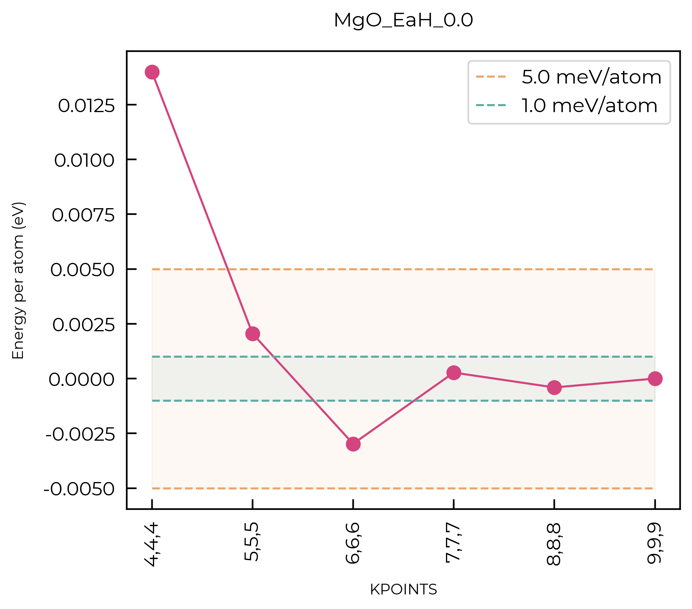
Mg_EaH_0.0:
fig = parse_kpoints(Mg_EaH_0_0, title="Mg_EaH_0.0")
Mg_EaH_0.0061:
fig = parse_kpoints(Mg_EaH_0_0061, title="Mg_EaH_0.0061")
Mg_EaH_0.0099:
fig = parse_kpoints(Mg_EaH_0_0099, title="Mg_EaH_0.0099")
So the converged values are:
MgO:
k8x8x8(used before)Mg_EaH_0.0:
k7x7x7Mg_EaH_0.0061:
k9x9x5Mg_EaH_0.0099:
k7x7x2
6.1.2 Relaxations of competing phases
Next, you want to relax each competing phase with the converged k-point mesh, and calculate the energy with the same DFT functional and settings as your defect supercell calculations. doped can generate these folders for the relaxations of the competing phases.
The k-point meshes are Γ-centred (as opposed to Monkhorst-Pack) by default. By default doped will
make the inputs assuming a HSE06 INCAR (see HSESet.yaml for default values) and kpoint densities of 95 kpoints/Å3 for metals and 45 kpoints/Å3 for semiconductors.
Since in this qualitative tutorial we’re using PBEsol, we’ll update the INCAR settings to use this functional.
In addition, you should change the KPOINTS file to match the converged mesh in each case, however the default densities are good starting points. doped will automatically set SIGMA and ISMEAR accordingly depending on whether the phase is a semiconductor or metal, and will set NUPDOWN appropriately for molecules (i.e. O2 has triplet spin).
These relaxations can be set up with:
user_incar_settings = {
    "ENCUT": 1.3*450, # converged value for bulk MgO multiplied by 1.3 to account for Pulay stress during volume relaxation
    "GGA": "PS", # PBEsol
    "LHFCALC": False, # no hybrid functional
    "AEXX": 0.0, # no hybrid functional
    "HFSCREEN": 0.0, # no hybrid functional
    "NCORE": 8, # Update to the correct value for your HPC!
    "NELM": 120, # Increase NELM for metals
}
cp.vasp_std_setup(  # now renamed to `write_relaxation_files`
    user_incar_settings=user_incar_settings,
    # potcar_spec=True  # uncomment to run on Colab!
)
`CompetingPhases.vasp_std_setup` is deprecated and will be removed in the next minor release (v4.1); use `CompetingPhases.write_relaxation_files` instead.
{'CompetingPhases/MgO_Fm-3m_EaH_0/Relax': doped DopedDictSet with structure composition Mg1 O1. Available attributes:
 {'prev_vasprun', 'auto_metal_kpoints', 'vdw', 'potcar_functional', 'sym_prec', 'structure', 'user_potcar_settings', 'kpoints', 'charge_state', 'validate_magmom', 'incar', 'user_kpoints_settings', 'nelect', 'use_structure_charge', 'prev_incar', 'potcar', 'constrain_total_magmom', 'reduce_structure', 'auto_kpar', 'force_gamma', 'poscar', 'kpoints_updates', 'auto_kspacing', 'sort_structure', 'standardize', 'potcar_symbols', 'incar_updates', 'config_dict', 'user_incar_settings', 'prev_kpoints', 'user_potcar_functional', 'files_to_transfer', 'international_monoclinic', 'auto_ispin', 'prev_outcar', 'auto_ismear', 'bandgap', 'poscar_comment', 'inherit_incar', 'auto_lreal', 'bandgap_tol'}

 Available methods:
 {'load', 'unsafe_hash', 'from_directory', 'get_input_set', 'validate_monty_v1', 'write_input', 'calculate_ng', 'validate_monty_v2', 'as_dict', 'save', 'override_from_prev_calc', 'get_vasp_input', 'estimate_nbands', 'to_json', 'from_dict', 'from_prev_calc'},
 'CompetingPhases/Mg_P6_3mmc_EaH_0/Relax': doped DopedDictSet with structure composition Mg2. Available attributes:
 {'prev_vasprun', 'auto_metal_kpoints', 'vdw', 'potcar_functional', 'sym_prec', 'structure', 'user_potcar_settings', 'kpoints', 'charge_state', 'validate_magmom', 'incar', 'user_kpoints_settings', 'nelect', 'use_structure_charge', 'prev_incar', 'potcar', 'constrain_total_magmom', 'reduce_structure', 'auto_kpar', 'force_gamma', 'poscar', 'kpoints_updates', 'auto_kspacing', 'sort_structure', 'standardize', 'potcar_symbols', 'incar_updates', 'config_dict', 'user_incar_settings', 'prev_kpoints', 'user_potcar_functional', 'files_to_transfer', 'international_monoclinic', 'auto_ispin', 'prev_outcar', 'auto_ismear', 'bandgap', 'poscar_comment', 'inherit_incar', 'auto_lreal', 'bandgap_tol'}

 Available methods:
 {'load', 'unsafe_hash', 'from_directory', 'get_input_set', 'validate_monty_v1', 'write_input', 'calculate_ng', 'validate_monty_v2', 'as_dict', 'save', 'override_from_prev_calc', 'get_vasp_input', 'estimate_nbands', 'to_json', 'from_dict', 'from_prev_calc'},
 'CompetingPhases/Mg_R-3m_EaH_0.003/Relax': doped DopedDictSet with structure composition Mg3. Available attributes:
 {'prev_vasprun', 'auto_metal_kpoints', 'vdw', 'potcar_functional', 'sym_prec', 'structure', 'user_potcar_settings', 'kpoints', 'charge_state', 'validate_magmom', 'incar', 'user_kpoints_settings', 'nelect', 'use_structure_charge', 'prev_incar', 'potcar', 'constrain_total_magmom', 'reduce_structure', 'auto_kpar', 'force_gamma', 'poscar', 'kpoints_updates', 'auto_kspacing', 'sort_structure', 'standardize', 'potcar_symbols', 'incar_updates', 'config_dict', 'user_incar_settings', 'prev_kpoints', 'user_potcar_functional', 'files_to_transfer', 'international_monoclinic', 'auto_ispin', 'prev_outcar', 'auto_ismear', 'bandgap', 'poscar_comment', 'inherit_incar', 'auto_lreal', 'bandgap_tol'}

 Available methods:
 {'load', 'unsafe_hash', 'from_directory', 'get_input_set', 'validate_monty_v1', 'write_input', 'calculate_ng', 'validate_monty_v2', 'as_dict', 'save', 'override_from_prev_calc', 'get_vasp_input', 'estimate_nbands', 'to_json', 'from_dict', 'from_prev_calc'},
 'CompetingPhases/Mg_P6_3mmc_EaH_0.009/Relax': doped DopedDictSet with structure composition Mg4. Available attributes:
 {'prev_vasprun', 'auto_metal_kpoints', 'vdw', 'potcar_functional', 'sym_prec', 'structure', 'user_potcar_settings', 'kpoints', 'charge_state', 'validate_magmom', 'incar', 'user_kpoints_settings', 'nelect', 'use_structure_charge', 'prev_incar', 'potcar', 'constrain_total_magmom', 'reduce_structure', 'auto_kpar', 'force_gamma', 'poscar', 'kpoints_updates', 'auto_kspacing', 'sort_structure', 'standardize', 'potcar_symbols', 'incar_updates', 'config_dict', 'user_incar_settings', 'prev_kpoints', 'user_potcar_functional', 'files_to_transfer', 'international_monoclinic', 'auto_ispin', 'prev_outcar', 'auto_ismear', 'bandgap', 'poscar_comment', 'inherit_incar', 'auto_lreal', 'bandgap_tol'}

 Available methods:
 {'load', 'unsafe_hash', 'from_directory', 'get_input_set', 'validate_monty_v1', 'write_input', 'calculate_ng', 'validate_monty_v2', 'as_dict', 'save', 'override_from_prev_calc', 'get_vasp_input', 'estimate_nbands', 'to_json', 'from_dict', 'from_prev_calc'},
 'CompetingPhases/O2_mmm_EaH_0/Relax': doped DopedDictSet with structure composition O2. Available attributes:
 {'prev_vasprun', 'auto_metal_kpoints', 'vdw', 'potcar_functional', 'sym_prec', 'structure', 'user_potcar_settings', 'kpoints', 'charge_state', 'validate_magmom', 'incar', 'user_kpoints_settings', 'nelect', 'use_structure_charge', 'prev_incar', 'potcar', 'constrain_total_magmom', 'reduce_structure', 'auto_kpar', 'force_gamma', 'poscar', 'kpoints_updates', 'auto_kspacing', 'sort_structure', 'standardize', 'potcar_symbols', 'incar_updates', 'config_dict', 'user_incar_settings', 'prev_kpoints', 'user_potcar_functional', 'files_to_transfer', 'international_monoclinic', 'auto_ispin', 'prev_outcar', 'auto_ismear', 'bandgap', 'poscar_comment', 'inherit_incar', 'auto_lreal', 'bandgap_tol'}

 Available methods:
 {'load', 'unsafe_hash', 'from_directory', 'get_input_set', 'validate_monty_v1', 'write_input', 'calculate_ng', 'validate_monty_v2', 'as_dict', 'save', 'override_from_prev_calc', 'get_vasp_input', 'estimate_nbands', 'to_json', 'from_dict', 'from_prev_calc'}}
Update the KPOINTS file to match the converged mesh in each case:
from pymatgen.io.vasp.inputs import Kpoints

converged_values = {"MgO_Fm-3m_EaH_0": (8,8,8), "Mg_Fm-3m_EaH_0": (7,7,7), "Mg_R-3m_EaH_0.003": (9,9,5), "Mg_P6_3mmc_EaH_0.009": (7,7,2)}

for k, v in converged_values.items():
    # Update KPOINTS
    path = f"CompetingPhases/{k}/vasp_std/KPOINTS"
    # Read KPOINTS
    kpoints = Kpoints(kpts=(v,))
    # Write file to path
    kpoints.write_file(path)
Remember that the final ENCUT used for the energy calculations should be the same as for your host
material & defects. To ensure this, after relaxing with 1.3*ENCUT, we resubmit a final quick relaxation with ENCUT.
6.2 Parse Competing Phases
Tip
See the main competing phases tutorial for more info.
6.2.1 Read in data from vasprun.xml files
Once you’ve calculated your competing phases, you will want to parse the results to determine the chemical potential limits of your host material. To do this, we need to parse the vasprun.xml files from your final
production-run competing phase calculations. To download the vasprun.xml files from the HPCs recursively, you can recursively rsync:
rsync -azvuR hpc:'path/to/the/base/folder/competing_phases/./*_EaH_*/vasp_std/vasprun.xml*' .
where the /./ indicates where you’d like to start the recurse from, so you only keep the folder structure from the <formula>_<space group>_EaH_* point onwards. If you’ve done spin-orbit coupling (SOC) calculations with results in vasp_ncl folders, then you need to change vasp_std to vasp_ncl above, or to whatever name you’ve given the production-run folders. Note that you can compress the vasprun.xml files to save space (with e.g. find . -name vasprun.xml -exec gzip {} \;) and these will still be parsed fine by doped.
All analysis is performed with the CompetingPhasesAnalyzer class, and all you need to supply it is the formula of your host system and the path to the base folder in which you have all your formula_EaH_*/<subfolder>/vasprun.xml(.gz) files.
from doped.chemical_potentials import CompetingPhasesAnalyzer
cpa = CompetingPhasesAnalyzer(composition="MgO", entries="MgO/CompetingPhases")
Parsing vaspruns...: 100%|██████████| 5/5 [00:00<00:00, 109.33it/s]
We see here that doped will automatically warn us if incompatible settings are used in our calculations, to reduce accidental errors. Of course if we generate all our input files through doped, this should never happen anyway (just shown here for illustration).
The chemical potential limits for our host material can then be obtained from cpa.chempots_df:
cpa.chempots_df
| Mg | O | |
|---|---|---|
| Limit | ||
| MgO-Mg | 0.00000 | -5.64572 |
| MgO-O2 | -5.64572 | 0.00000 |
To use these parsed chemical potential limits for computing the defect formation energies with doped (e.g. in plotting.formation_energy_plot(), analysis.formation_energy_table() etc.) we can use the cpa.chempots attribute, which is a dictionary of the chemical potential limits for each element in the host material:
cpa.chempots
{'limits': {'MgO-Mg': {'Mg': np.float64(-1.73606), 'O': np.float64(-10.78077)},
  'MgO-O2': {'Mg': np.float64(-7.38178), 'O': np.float64(-5.13505)}},
 'elemental_refs': {'O': -5.13505, 'Mg': -1.73606},
 'limits_wrt_el_refs': {'MgO-Mg': {'Mg': np.float64(0.0),
   'O': np.float64(-5.64572)},
  'MgO-O2': {'Mg': np.float64(-5.64572), 'O': np.float64(0.0)}}}
If you want to save it to use at a later date / in a different notebook/environment without having to re-parse your results, you can dump it to a json file with dumpfn and then load it again with loadfn:
from monty.serialization import dumpfn, loadfn

dumpfn(cpa.chempots, 'MgO/CompetingPhases/MgO_chempots.json')
MgO_chempots = loadfn('MgO/CompetingPhases/MgO_chempots.json')
6.3.1 Analyse and visualise the Chemical Potential Limits
from pymatgen.analysis.chempot_diagram import ChemicalPotentialDiagram

cpd = ChemicalPotentialDiagram(cpa.intrinsic_phase_diagram.entries)
plot = cpd.get_plot()
plot.show()
Because cpd.get_plot() returns a plotly object, it’s almost infinitely customisable using plot.update_scenes() - you can change colours, fonts, axes and even data after it’s been plotted. See the docs for more info.
Beware that because we only generated the relevant competing phases on the Mg-O phase diagram for our MgO host material, we have not calculated all phase in the Mg-O chemical space (just those that are necessary to determine the chemical potential limits of MgO), and so these chemical potential diagram plots are only accurate in the vicinity of our host material.
7. Dielectric constant
For single-crystal semiconductors, the response to a static electric field can be decomposed into two components:
\(\epsilon_{0} = \epsilon_{ionic} + \epsilon_{infinity}\)
where \(\epsilon_{ionic}\) is often called the low-frequency or ionic dielectric constant and \(\epsilon_{infinity}\) the high frequency or optical dielectric constant.
We’ll calculate both contributions below.
Important
The calculated value for the ionic contribution to the static dielectric constant (\(\epsilon_{ionic}\)) is quite sensitive to both the plane wave kinetic energy cutoff ENCUT and the k-point density, with more expensive parameter values necessary (relative to ground-state-energy-converged values) due to the requirement of accurate ionic forces. Thus, this calculation should be accompanied with convergence tests with respect to these parameters.
In addition, the calculation of the optical dielectric constant (\(\epsilon_{optical}\)) is sensitive to the number of electronic bands included in the calculation (NBANDS), and often requires a high value for convergence.
We can quickly perform these convergence tests with vaspup2.0, as shown below.
7.1 Optical contribution (\(\epsilon_{optical}\))
The optical contribution results from the refraction of electromagnetic waves with frequencies high compared to lattice vibrations (phonons). We can calculate the optical dielectric functions and take the value of the real component at E = 0 eV.
Important
Typically, we perform the convergence test of $\epsilon_{optical}$ with respect to the number of bands (NBANDS) using a GGA functional like PBEsol, and use the converged NBANDS to recalculate $\epsilon_{optical}$ with a hybrid functional, as explained here.
In this tutorial, we’re using PBEsol so we’ll just use the value from the convergence test below. But remember that in a typical study, you’d then use the converged NBANDS value for the hybrid functional calculation!
7.1.1 Convergence of NBANDS for \(\epsilon_{optical}\)
Generate input files for NBANDS convergence
We first generate the input files for the convergence tests and save them to a folder called Dielectric/Bulk_optical/Convergence/input:
import os

# Create directory for optical and convergence calcs
os.makedirs("MgO/Dielectric/Optical/Convergence/input", exist_ok=True)
#  Copy input files from bulk relaxation directory
import shutil
from pymatgen.core.structure import Structure

if not os.path.exists("./MgO/Bulk_relax/CONTCAR"):
    print("Please run the bulk relaxation first!")
else:
    shutil.copy("./MgO/Bulk_relax/CONTCAR", "./MgO/Dielectric/Optical/Convergence/input/POSCAR")

# Copy KPOINTS, POTCAR and INCAR
shutil.copy("./MgO/Bulk_relax/KPOINTS", "./MgO/Dielectric/Optical/Convergence/input/KPOINTS")
# comment this out on Colab; requires POTCARs setup with pymatgen; https://doped.readthedocs.io/en/latest/Installation.html
shutil.copy("./MgO/Bulk_relax/POTCAR", "./MgO/Dielectric/Optical/Convergence/input/POTCAR");
# INCAR for optical convergence
from pymatgen.io.vasp.inputs import Incar
incar = Incar.from_dict(
    {
        # System-dependent parameters
        "ENCUT": 450, # Converged value for your material
        # Optical parameters:
        'LOPTICS': True,
        'CSHIFT': 1e-06,
        'NBANDS': 120,
        'ISMEAR': -5, # Tetrahedron method
        'SIGMA': 0.05, # Smearing
        'NEDOS': 2000,
        'ALGO': 'Normal',
        'ISPIN': 2,
        'LORBIT': 11,
        'LREAL': False,
        # Electronic convergence (tight):
        'EDIFF': 1e-07,
        'NELM': 100,
        # Functional:
        'GGA': 'Ps', # For converging NBANDS we use PBEsol
        'PREC': 'Accurate',
        # Parallelisation:
        'KPAR': 2,
        'NCORE': 6,
    }
)
# Save to file
incar.write_file("./MgO/Dielectric/Optical/Convergence/input/INCAR")
To use vaspup2.0, we need to use a CONFIG file like the one below. Here we need to decide on the range on NBANDS to test. Typically, we our minimum value should be the number of valence electrons in the structure and go up to that ~number+200
# This cell will fail on Colab; requires POTCARs to be setup with `pymatgen` (https://doped.readthedocs.io/en/latest/Installation.html)
# Number of valence electrons in our system
from pymatgen.io.vasp.inputs import Potcar
from pymatgen.core.structure import Structure
from pymatgen.core.periodic_table import Element

potcar = Potcar.from_file("./MgO/Bulk_relax/POTCAR")
prim_struc = Structure.from_file("./MgO/Bulk_relax/CONTCAR")
d = prim_struc.composition.as_dict()
d_Z_to_num_atoms = {Element(e).Z: v for e, v in d.items()} # Map atomic number to number of atoms of that element in structure
# Get number of valence electrons in structure
n_elec = 0
for potcar_single in potcar:
    n_elec += potcar_single.nelectrons * d_Z_to_num_atoms[potcar_single.atomic_no] # number of electrons in potcar * number of atoms of that element in structure
print(f"Number of valence electrons: {n_elec}")
Number of valence electrons: 8.0
nbands_start = n_elec  # 8 (set manually on Colab)
nbands_end = nbands_start + 200
print(f"Start nbands: {nbands_start}. End nbands: {nbands_end}")
Start nbands: 8.0. End nbands: 208.0
config_file = f"""# vaspup2.0 Config file
# This is config for automating NBANDS convergence.
# (For LOPTICS calculation)(High-frequency dielectric constant)

conv_nbands="1"		# 1 for ON, 0 for OFF
nbands_start="{int(nbands_start)}"	# Value to start NBANDS calcs from
# Need to include NBANDS flag in INCAR
nbands_end="{int(nbands_end)}"		# Value to end NBANDS calcs on
nbands_step="20"		# NBANDS increment

run_vasp="1"		# Run VASP after generating the files? (1 for ON, 0 for OFF)
#name="Optical" # Optional name to append to each jobname (remove "#")
"""
# Save it to input
with open("./MgO/Dielectric/Optical/Convergence/input/CONFIG", "w") as f:
    f.write(config_file)
We transfer the input folder to the HPC and run the convergence tests with vaspup2.0 by running the command nbands-generate-converge from the directory above the input directory.
After the calculations finished, we can parse the results by executing the command nbands-epsopt-data-converge from the nbands_converge directory, which outputs:
NBANDS Convergence Results
# Output from vaspup2.0 nbands-converge
optical_conv = """
Directory:                   Epsilon_Opt X,Y,Z:                     Difference EpsOpt X,Y,Z:
nbands8         2.033336        2.033336        2.033336
nbands28        2.097091        2.097091        2.097091        0.0701           0.0701          0.0701
nbands48        2.100513        2.100513        2.100513        -0.0034          -0.0034         -0.0034
nbands68        2.103436        2.103436        2.103436        -0.0029          -0.0029         -0.0029
nbands88        2.101419        2.101419        2.101419        -0.0681          -0.0681         -0.0681
nbands_108      2.102865        2.102865        2.102865        -0.0014          -0.0014         -0.0014
nbands_128      2.102674        2.102674        2.102674        0.0002           0.0002          0.0002
nbands_148      2.103785        2.103785        2.103785        -0.0011          -0.0011         -0.0011
nbands_168      2.104084        2.104084        2.104084        -0.0003          -0.0003         -0.0003
nbands_188      2.102393        2.102393        2.102393        0.0017           0.0017          0.0017
nbands_208      2.103104        2.103104        2.103104        -0.0007          -0.0007         -0.0007
"""
We can plot it to see the convergence:
# Parse x,y,z values from optical convergence
optical_conv = optical_conv.split("\n")[1:]
optical_conv = [line.split() for line in optical_conv][1:-1]
nbands = [int(line[0].split("nbands")[1].split("_")[-1]) for line in optical_conv]
optical_conv = [line[1:4] for line in optical_conv]
# print(optical_conv)
# Plot x,y,z values in different subplots
import matplotlib.pyplot as plt
import numpy as np
fig, axs = plt.subplots(3, sharex=True, sharey=True)
fig.suptitle('Optical convergence')
axs[0].plot(nbands, [float(line[0]) for line in optical_conv], marker="o")
axs[0].set_ylabel("X")
axs[1].plot(nbands, [float(line[1]) for line in optical_conv], marker="o")
axs[1].set_ylabel("Y")
axs[2].plot(nbands, [float(line[2]) for line in optical_conv], marker="o")
axs[2].set_ylabel("Z")
axs[2].set_xlabel("NBANDS")
# Horizontal lines +-1% of last value
for i in range(3):
    axs[i].hlines(
        y=1.01 * float(optical_conv[-1][i]),
        xmin=nbands[0],
        xmax=nbands[-1],
        color="red",
        linestyles="dashed",
    )
    axs[i].hlines(
        y=0.99 * float(optical_conv[-1][i]),
        xmin=nbands[0],
        xmax=nbands[-1],
        color="red",
        linestyles="dashed",
    )
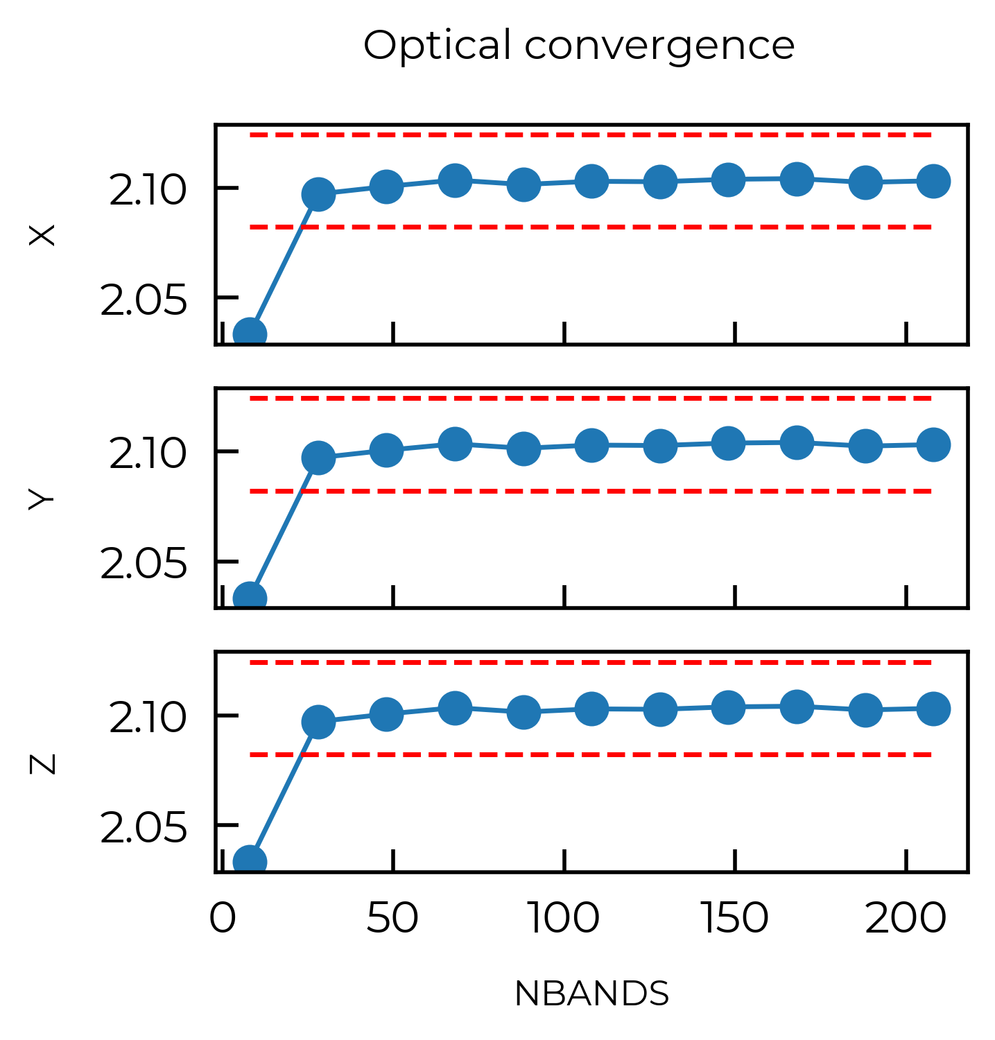
Which shows that with NBANDS = 28 (second point in the plot), $\epsilon_{optical}$ is within 1% of the converged value.
# Values for nbands = 28
index = nbands.index(28)
# Values of epsilon_opt for nbands = 28
epsilon_optical_converged = [float(line) for line in optical_conv[index]]
print(f"Converged Epsilon_optical: {epsilon_optical_converged}")
Converged Epsilon_optical: [2.097091, 2.097091, 2.097091]
Tip
Note that in a proper defect study, you’d know recompute $\epsilon_{optical}$ with a hybrid functional (e.g. HSE06), using the converged NBANDS value from the (PBEsol) convergence test above.
This is important, since this calculation is very sensitive to the band gap. Since LDA/GGA typically underestimates the band gap, the resulting dielectric constant is overestimated.
You could set the input for that calculation it with the following (commented) cell:
#  Copy input files from bulk relaxation directory
import shutil
from pymatgen.core.structure import Structure
from pymatgen.io.vasp.inputs import Incar, Kpoints, Potcar, VaspInput

if not os.path.exists("./MgO/Bulk_relax/CONTCAR"):
    print("Please run the bulk relaxation first!")
else:
    shutil.copy("./MgO/Bulk_relax/CONTCAR", "./MgO/Dielectric/Optical/Hybrid/POSCAR")

# Copy KPOINTS, POTCAR and INCAR
shutil.copy("./MgO/Bulk_relax/KPOINTS", "./MgO/Dielectric/Optical/Hybrid/KPOINTS")
# comment this out on Colab; requires POTCARs setup with pymatgen; https://doped.readthedocs.io/en/latest/Installation.html
shutil.copy("./MgO/Bulk_relax/POTCAR", "./MgO/Dielectric/Optical/Hybrid/POTCAR")
# Incar file
incar = Incar.from_file("./MgO/Dielectric/Optical/Convergence/input/INCAR")
incar.update(
    {
        "NBANDS": 28, # underlying GGA functional for HSE/PBE0 is PBE
        # Functional:
        "GGA": "PE",
        "LHFCALC": True,
        "AEXX": 0.25,  # HSE06 assumed by default. Set AEXX in INCAR config settings to tune alpha xc parameter.
        "HFSCREEN": 0.208,  # correct HSE screening parameter; see https://aip.scitation.org/doi/10.1063/1.2404663
        "PRECFOCK": "Fast",
        # Paralelisation:
        "NCORE": 8, # Might need updating for your HPC!
        "KPAR": 2,
    }
)
print("Incar settings for hyrbid calculation of E_optical:", incar)
# Save file
incar.write_file("./MgO/Dielectric/Optical/Optical/Hybrid/INCAR")
7.2 Ionic contribution (\(\epsilon_{ionic}\))
To calculate the low-frequency behaviour, we need to compute the response of the lattice vibrations (phonons) to an applied electric field.
Important
Typically, \(\epsilon_{ionic}\) is calculated with PBEsol, since this functional is accurate for phonons (and thus \(\epsilon_{ionic}\)).
Accordingly, in a typical defect stude we use a hybrid functional (e.g. HSE06) for our bulk/defect calculations and for \(\epsilon_{optical}\), and PBEsol for \(\epsilon_{ionic}\), e.g.:
\( \epsilon_0 = \epsilon_{optical}\) (from hybrid optics calc) \(+ \epsilon_{ionic}\) (from PBEsol DFPT)
But remember that if you’re changing functional (e.g. if you’ve used HSE06 to relax your bulk structure and now you’ll use PBEsol to calculate \(\epsilon_{ionic}\)), you first have to re-relax the bulk structure again with PBEsol before calculating \(\epsilon_{ionic}\) with PBEsol!
Note
In addition, note that the calculation of $\epsilon_{ionic}$ is very sensitive to the input geometry, and requires a well converged relaxed structure. Otherwise, negative phonon modes can give unreasonably large values of the ionic response. Thus, we’ll perform a very tight relaxation of our primitive structure (e.g. EDIFFG = -1E-6 and EDIFF = 1E-8).
7.2.1 Tight relaxation
#  Copy input files from bulk relaxation directory
import shutil
from pymatgen.core.structure import Structure
import os

# Create directory
os.makedirs("MgO/Dielectric/Ionic/Relax_tight", exist_ok=True)

if not os.path.exists("./MgO/Bulk_relax/CONTCAR"):
    print("Please run the bulk relaxation first!")
else:
    shutil.copy("./MgO/Bulk_relax/CONTCAR", "./MgO/Dielectric/Ionic/Relax_tight/POSCAR")

# Copy KPOINTS, POTCAR and INCAR
shutil.copy("./MgO/Bulk_relax/KPOINTS", "./MgO/Dielectric/Ionic/Relax_tight/KPOINTS")
# comment this out on Colab; requires POTCARs setup with pymatgen; https://doped.readthedocs.io/en/latest/Installation.html
shutil.copy("./MgO/Bulk_relax/POTCAR", "./MgO/Dielectric/Ionic/Relax_tight/POTCAR");
incar = Incar.from_file("./MgO/Input_files/INCAR_bulk_relax")
incar.update(
    {
        "ENCUT": 450 * 1.3, # Increase ENCUT by 30% because we're relaxing volume (Pulay stress)
        # Paralelisation
        "KPAR": 2,
        "NCORE": 8, # Might need updating for your HPC!
        # Functional
        "GGA": "PS",
        # Relaxation
        "IBRION": 2,
        "ISIF": 3, # Relax cell
        "NSW": 800, # Max number of steps
        # Accuracy and thresholds
        "ISYM": 2, # Symmetry on
        "PREC": "Accurate",
        "EDIFF": 1e-8, # Tight electronic convergence
        "EDIFFG": -1e-4, # Tight ionic convergence
        "ALGO": "Normal",
        "LREAL": "False",
    }
)
# Save to file
incar.write_file("./MgO/Dielectric/Ionic/Relax_tight/INCAR")
After the relaxation finished, we copy the CONTCAR from the HPC to the current directory and parse it with pymatgen:
If we also transfer the vasprun.xml file we can check the relaxation is converged like:
import os

if os.path.exists("./MgO/Dielectric/Ionic/Relax_tight/CONTCAR"):
    prim_struc_tight = Structure.from_file("./MgO/Dielectric/Ionic/Relax_tight/CONTCAR")
else:
    print(f"Perform the relaxation first!")
from pymatgen.io.vasp.outputs import Vasprun

# Can check if relaxation is converged by parsing the vasprun.xml
if os.path.exists("MgO/Dielectric/Ionic/Relax_tight/vasprun.xml.gz"):
    vr = Vasprun("MgO/Dielectric/Ionic/Relax_tight/vasprun.xml.gz")
    print(f"Relaxation converged?", vr.converged)
else:
    print(f"No vasprun.xml found!")
Relaxation converged? True
7.2.2 Convergence of ENCUT and kpoints for \(\epsilon_{ionic}\)
Generate input files for ENCUT/KPOINTS convergence
import os

# Create directory for optical and convergence calcs
os.makedirs("MgO/Dielectric/Ionic/Convergence/input", exist_ok=True)
#  Copy input files from bulk relaxation directory
import shutil
from pymatgen.core.structure import Structure

if not os.path.exists("./MgO/Dielectric/Ionic/Relax_tight/CONTCAR"):
    print("Please run the tight bulk relaxation first!")
else:
    shutil.copy("./MgO/Dielectric/Ionic/Relax_tight/CONTCAR", "./MgO/Dielectric/Ionic/Convergence/input/POSCAR")

# Copy KPOINTS, POTCAR and INCAR
shutil.copy("./MgO/Bulk_relax/KPOINTS", "./MgO/Dielectric/Ionic/Convergence/input/KPOINTS")
# comment this out on Colab; requires POTCARs setup with pymatgen; https://doped.readthedocs.io/en/latest/Installation.html
shutil.copy("./MgO/Bulk_relax/POTCAR", "./MgO/Dielectric/Ionic/Convergence/input/POTCAR");
# INCAR for optical convergence
from pymatgen.io.vasp.inputs import Incar
incar = Incar.from_dict(
    {
        # System-dependent parameters
        "ENCUT": 450, # Converged value for your material
        # Parameters to calculated ionic dielectric constant:
        'LEPSILON': True, # DFPT Calculation
        'IBRION': 8, # Phonons
        'ISYM': -1, # Symmetry off (if using NCORE)
        'EDIFFG': -0.003,
        'ISIF': 2, # Keep cell volume fixed for DFPT calcs
        'NSW': 1,
        'LWAVE': True,
        # Electronic convergence:
        'EDIFF': 1e-07,
        'ALGO': 'Normal',
        'NELM': 100,
        'ISMEAR': 0, # Gaussian smearing
        'SIGMA': 0.05,
        'NEDOS': 2000,
        'ISPIN': 1, # off for non-magnetic systems
        # Others:
        'LREAL': False,
        'LORBIT': 11,
        'LASPH': True,
        # Functional:
        'GGA': 'Ps',
        'PREC': 'Accurate',
        # Parallelisation:
        'KPAR': 2,
        'NCORE': 8,
    }
)
# Save to file
incar.write_file("./MgO/Dielectric/Ionic/Convergence/input/INCAR")
And finally we set the kpoint meshes that we’ll try in the CONFIG file. We can get a list of of kpoint grids for our system by using the kgrid package (which can be installed by running pip install kgrid):
from kgrid.series import cutoff_series
from kgrid import calc_kpt_tuple
import numpy as np
from pymatgen.core.structure import Structure
from pymatgen.io.ase import AseAtomsAdaptor

def generate_kgrids_cutoffs(
    structure: Structure,
    kmin: int = 4,
    kmax: int = 20,
) -> list:
    """Generate a series of kgrids for your lattice between a real-space cutoff range of `kmin` and `kmax` (in A).
    For semiconductors, the default values (kmin: 4; kmax: 20) are generally good.
    For metals you might consider increasing a bit the cutoff (kmax~30).
    Returns a list of kmeshes.
    Args:
        atoms (ase.atoms.Atoms): _description_
        kmin (int, optional): _description_. Defaults to 4.
        kmax (int, optional): _description_. Defaults to 20.

    Returns:
        list: list of kgrids
    """
    # Transform struct to atoms
    aaa = AseAtomsAdaptor()
    atoms = aaa.get_atoms(structure=structure)
    # Calculate kgrid samples for the given material
    kpoint_cutoffs = cutoff_series(
        atoms=atoms,
        l_min=kmin,
        l_max=kmax,
    )
    kgrid_samples = [
        calc_kpt_tuple(atoms, cutoff_length=(cutoff - 1e-4))
        for cutoff in kpoint_cutoffs
    ]
    print(f"Kgrid samples: {kgrid_samples}")

    return kgrid_samples
from pymatgen.core.structure import Structure

prim_struc = Structure.from_file("MgO/Bulk_relax/CONTCAR")
kgrids = generate_kgrids_cutoffs(prim_struc)
kgrids = list(set(kgrids)) # Avoid duplicates
# Sort
kgrids.sort()
# # As string, to copy to vaspup2.0 CONFIG file
kpoints_string = ""
for k in kgrids:
    kpoints_string += f"{k[0]} {k[1]} {k[2]},"
kpoints_string
Kgrid samples: [(4, 4, 4), (5, 5, 5), (6, 6, 6), (7, 7, 7), (8, 8, 8), (9, 9, 9), (10, 10, 10), (11, 11, 11), (12, 12, 12), (13, 13, 13), (14, 14, 14), (15, 15, 15), (16, 16, 16)]
'4 4 4,5 5 5,6 6 6,7 7 7,8 8 8,9 9 9,10 10 10,11 11 11,12 12 12,13 13 13,14 14 14,15 15 15,16 16 16,'
config=f"""# vaspup2.0 Config File
# This is the default config for automating convergence.
# Works for ground-state energy convergence and DFPT convergence.

conv_encut="1"		# 1 for ON, 0 for OFF (ENCUT Convergence Testing)
encut_start="300"	# Value to start ENCUT calcs from.
encut_end="900"		# Value to end ENCUT calcs on.
encut_step="50"		# ENCUT increment.

conv_kpoint="1"		# 1 for ON, 0 for OFF (KPOINTS Convergence Testing)
kpoints="{kpoints_string}" # All the kpoints meshes
# you want to try, separated by a comma

run_vasp="1"		# Run VASP after generating the files? (1 for ON, 0 for OFF)
#name="DFPT" # Optional name to append to each jobname (remove "#")
"""
# Save it to input directory
with open("./MgO/Dielectric/Ionic/Convergence/input/CONFIG", "w") as f:
    f.write(config)
After the calculations finish we can run dfpt-data-converge in the cutoff_converge and kpoint_converge directories to parse the results:
ENCUT Dielectric Convergence Results
ionic_encut_str="""
Directory:               Epsilon 100,010,001:                     Difference 100,010,001:
e300            6.411938        6.411951        6.411951
e350            6.649273        6.649267        6.649273        -0.2373          -0.2373         -0.2373
e400            6.828065        6.828061        6.828065        -0.1788          -0.1788         -0.1788
e450            6.805369        6.805371        6.805390        0.0227           0.0227          0.0227
e500            6.818039        6.818043        6.818032        -0.0127          -0.0127         -0.0126
e550            6.814258        6.814268        6.814261        0.0038           0.0038          0.0038
e600            6.818120        6.818120        6.818116        -0.0039          -0.0039         -0.0039
e650            6.850394        6.850393        6.850403        -0.0323          -0.0323         -0.0323
e700            6.859188        6.859174        6.858902        -0.0088          -0.0088         -0.0085
e750            6.864191        6.863926        6.863944        -0.0050          -0.0048         -0.0050
e800            6.866957        6.866955        6.866964        -0.0028          -0.0030         -0.0030
e850            6.867236        6.867240        6.867218        -0.0003          -0.0003         -0.0003
e900            6.862659        6.862657        6.862674        0.0046           0.0046          0.0045
"""
ionic_kpoint_str="""
Directory:               Epsilon 100,010,001:                     Difference 100,010,001:
k4,4,4          7.157532        7.157509        7.157532
k5,5,5          6.889848        6.889842        6.889834        0.2677           0.2677          0.2677
k6,6,6          6.822478        6.822475        6.822464        0.0674           0.0674          0.0674
k7,7,7          6.805369        6.805371        6.805390        0.0171           0.0171          0.0171
k8,8,8          6.800997        6.800992        6.801008        0.0044           0.0044          0.0044
k9,9,9          6.799887        6.799889        6.799889        0.0011           0.0011          0.0011
k_10,10,10      6.799197        6.799197        6.799202        0.0007           0.0007          0.0007
k_11,11,11      6.799392        6.799393        6.799397        -0.0002          -0.0002         -0.0002
k_12,12,12      6.799260        6.799248        6.799270        0.0001           0.0001          0.0001
k_13,13,13      6.799323        6.799327        6.799331        -0.0001          -0.0001         -0.0001
k_14,14,14      6.799111        6.799112        6.799113        0.0002           0.0002          0.0002
k_15,15,15      6.799089        6.799088        6.799096        0.0000           0.0000          0.0000
k_16,16,16      6.799236        6.799239        6.799244        -0.0001          -0.0002         -0.0001
"""
And we can plot the convergence:
# Parse x,y,z values from optical convergence
ionic_encut = ionic_encut_str.split("\n")[1:]
ionic_encut = [line.split() for line in ionic_encut][1:-1]
encuts = [int(line[0].split("e")[1]) for line in ionic_encut]
# print("Encuts:", encuts)
ionic_encut = [line[1:4] for line in ionic_encut]
# print("Epsilon:", ionic_encut)
# print(optical_conv)
# Plot x,y,z values in different subplots
import matplotlib.pyplot as plt
import numpy as np
fig, axs = plt.subplots(3, sharex=True, sharey=True)
fig.suptitle('$\epsilon_{ionic}$ convergence wrt to ENCUT')
axs[0].plot(encuts, [float(line[0]) for line in ionic_encut], marker="o")
axs[0].set_ylabel("X")
axs[1].plot(encuts, [float(line[1]) for line in ionic_encut], marker="o")
axs[1].set_ylabel("Y")
axs[2].plot(encuts, [float(line[2]) for line in ionic_encut], marker="o")
axs[2].set_ylabel("Z")
axs[2].set_xlabel("Encut (eV)")
# Horizontal lines +-1% of last value
for i in range(3):
    axs[i].hlines(
        y=1.01 * float(ionic_encut[-1][i]),
        xmin=encuts[0],
        xmax=encuts[-1],
        color="red",
        linestyles="dashed",
    )
    axs[i].hlines(
        y=0.99 * float(ionic_encut[-1][i]),
        xmin=encuts[0],
        xmax=encuts[-1],
        color="red",
        linestyles="dashed",
    )
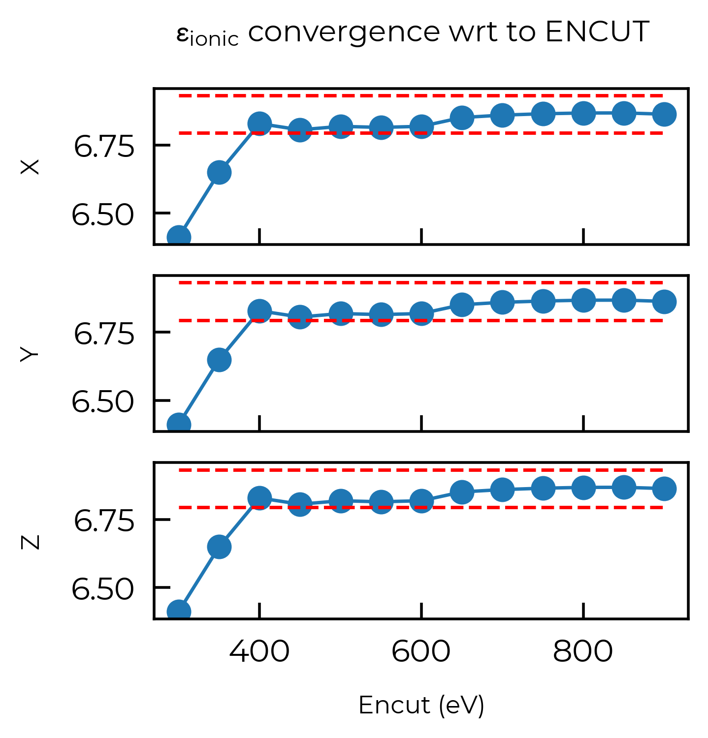
# Parse x,y,z values from optical convergence
data = ionic_kpoint_str.split("\n")[1:]
data = [line.split() for line in data][1:-1]
x = [line[0].split("k")[1].split("_")[-1].split()[0] for line in data]
# print("Encuts:", encuts)
data = [line[1:4] for line in data]
# print("Epsilon:", data)
# print(optical_conv)
# Plot x,y,z values in different subplots
import matplotlib.pyplot as plt
import numpy as np
fig, axs = plt.subplots(3, sharex=True, sharey=True)
fig.suptitle('$\epsilon_{ionic}$ convergence wrt to kpoints')
axs[0].plot(x, [float(line[0]) for line in data], marker="o")
axs[0].set_ylabel("X")
axs[1].plot(x, [float(line[1]) for line in data], marker="o")
axs[1].set_ylabel("Y")
axs[2].plot(x, [float(line[2]) for line in data], marker="o")
axs[2].set_ylabel("Z")
axs[2].set_xlabel("Kgrid")
# Horizontal lines +-1% of last value
for i in range(3):
    axs[i].hlines(
        y=1.01 * float(data[-1][i]),
        xmin=x[0],
        xmax=x[-1],
        color="red",
        linestyles="dashed",
    )
    axs[i].hlines(
        y=0.99 * float(data[-1][i]),
        xmin=x[0],
        xmax=x[-1],
        color="red",
        linestyles="dashed",
    )
# Rotate xtick labels
plt.xticks(rotation=90);
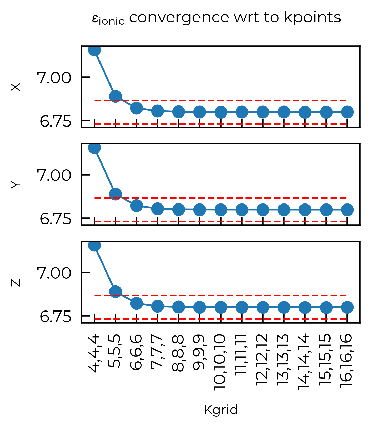
We see that for ENCUT=400 and kgrid=(6,6,6), \(\epsilon_{ionic}\) is within 1% of the converged value.
Since for the kpoint convergence, we used an ENCUT=450, we can take the value of \(\epsilon_{ionic}\) from the kgrid=(16,16,16) calculation. But note that this is not typically the case, where you should do a final calculation with the converged ENCUT value and kgrid.
# Print last value of epsilon in data
epsilon_ionic_converged = [float(line) for line in data[-1]]
print(f"Converged ionic epsilon: {epsilon_ionic_converged}")
Converged ionic epsilon: [6.799236, 6.799239, 6.799244]
7.3 Total dielectric (\(\epsilon_{total}\))
print(f"Converged ionic dielectric: {epsilon_ionic_converged}")
print(f"Converged optical dielectric: {epsilon_optical_converged}")

total_dielectric = np.array(epsilon_ionic_converged) + np.array(epsilon_optical_converged)
print(f"Converged total dielectric: {total_dielectric}")
Converged ionic dielectric: [6.799236, 6.799239, 6.799244]
Converged optical dielectric: [2.097091, 2.097091, 2.097091]
Converged total dielectric: [8.896327 8.89633  8.896335]
8. Density of States (DOS)
For thermodynamic / defect concentration analyses (shown later in this tutorial, see the Self-consistent Fermi level & carrier concentrations section), we need the bulk electronic density of states (DOS) in order to compute the electron and hole carrier concentrations (and thus the self-consistent Fermi levels).
This should be a static calculation on the primitive bulk unit cell, ideally using:
Tetrahedron smearing (
ISMEAR = -5) for improved DOS convergence with respect tok-points,Dense
k-point sampling and energy grid (NEDOS) for a well-converged DOS and accurate band gap,Consistent functional, pseudopotentials (
POTCARs),ENCUTand crystal structure as used for the bulk/defect supercell calculations.
Tip
See the DOS calculation tips in the doped documentation for more details and guidance.
from pymatgen.io.vasp.sets import MPStaticSet
from pymatgen.core.structure import Structure

# load the relaxed primitive bulk structure (from the bulk relaxation in Section 2):
prim_struc = Structure.from_file("./MgO/Bulk_relax/CONTCAR")

# `MPStaticSet` sets up a static calculation, and conveniently already uses tetrahedron
# smearing (`ISMEAR = -5`) and writes the orbital-projected DOS (`LORBIT = 11`) by default.
# We just increase `NEDOS` and the k-point density for a well-resolved, converged DOS:
dos_set = MPStaticSet(
    prim_struc,
    user_incar_settings={
        "NEDOS": 3000,    # dense energy grid for a well-resolved DOS
        "EDIFF": 1e-6,    # tight electronic convergence
        "ENCUT": 450,     # use the SAME ENCUT as your bulk/defect supercell calcs!
        "ISMEAR": -5,     # tetrahedron smearing (already the default here)
        # also match any settings (e.g. LHFCALC, AEXX, GGA, ...) used for
        # your supercell calculations, for consistency
        "GGA": "PS",  # Functional (PBEsol for this tutorial)
        "LHFCALC": False, # Disable Hybrid functional
        "NCORE": 8, # Parallelisation, might need updating for your HPC!
    },
    reciprocal_density=400,  # dense k-points; should be converged (e.g. with vaspup2.0)
    user_potcar_functional="PBE_54",
)
# write the VASP input files (POTCAR generation requires pymatgen POTCAR setup;
# https://doped.readthedocs.io/en/latest/Installation.html -- comment out, or pass
# `potcar_spec=True`, on Colab):
dos_set.write_input("MgO/Bulk_DOS")
!ls MgO/Bulk_DOS # DOS calculation input files
INCAR KPOINTS POSCAR POTCAR
After running this calculation, the resulting vasprun.xml(.gz) is the bulk DOS output that we provide as bulk_dos in the thermodynamic analyses below (here saved as MgO/MgO_DOS_vasprun.xml.gz). doped will warn you if the VBM eigenvalue or band gap of the bulk DOS differs significantly from that of the bulk/defect supercell calculations, which can indicate inconsistent settings (see the DOS calculation tips).
9. Defect analysis
9.1 Parse defect calculations
For parsing defect calculation results with doped, we need the following VASP output files
from our bulk and defect supercell calculations:
vasprun.xml(.gz)Either:
OUTCAR(.gz), if using the Kumagai-Oba (eFNV) charge correction scheme (compatible with isotropic or anisotropic (non-cubic) dielectric constants; recommended), orLOCPOT(.gz), if using the Freysoldt (FNV) charge correction scheme (isotropic dielectric screening only).
Note that doped can read the compressed versions of these files (.gz/.xz/.bz/.lzma), so we can
do e.g. gzip OUTCAR to reduce the file sizes when downloading and storing these files on our local
system.
To quickly compress these output files on our HPC, we can run the following from our top-level folder
containing the defect directories (e.g. Mg_O_0 etc):
for defect_dir in */vasp_*; do cd $defect_dir; gzip vasprun.xml OUTCAR; cd ../..; done
(change OUTCAR to LOCPOT if using the FNV isotropic charge correction), and then download the files
to the relevant folders by running the following from our local system:
for defect_dir in */vasp_*; do cd $defect_dir;
scp [remote_machine]:[path to doped folders]/${defect_dir}/\*gz .;
cd ../..; done
changing [remote_machine] and [path to doped folders] accordingly.
Note
If you want to use the example outputs shown in this parsing tutorial, you can do so by cloning the doped GitHub repository and following the dope_gga_workflow.ipynb Jupyter notebook.
!cp -r MgO/Defects/Pre_Calculated_Results/* MgO/Defects/  # copy in our pre-calculated example data
# comment this out if you have performed the DFT calculations yourself!
from doped.analysis import DefectsParser
%matplotlib inline
bulk_path = "./MgO/Defects/MgO_bulk/vasp_std"  # path to our bulk supercell calculation
dielectric = 8.8963 # dielectric constant (this can be a single number (isotropic), or a 3x1 array or 3x3 matrix (anisotropic))
dp = DefectsParser(
    output_path="MgO/Defects/",  # directory containing the defect calculation folders
    dielectric=dielectric,  # dielectric needed for charge corrections
    # processes=1,  # Can set the number of processes to 1 if you're having issues with multiprocessing
)
Parsing bulk reference calculation: 0%| | 0/5 [00:00<?, ?it/s]
Parsed Mg_O_+3/vasp_std: 100%|██████████| 5/5 [00:14<00:00, 2.98s/it]
DefectsParser uses multiprocessing by default to speed up parsing when we have many defect supercell calculations to parse. As described in its docstring shown below, it automatically searches the supplied output_path for the bulk and defect supercell calculation folders, then automatically determines the defect types, sites (from the relaxed structures) and charge states.
It also checks that appropriate INCAR, KPOINTS, POTCAR settings have been used, and will warn you if it detects any differences that could affect the defect formation energies.
Here we are warned that multiple vasprun.xml files were present in two of our directories (due to performing multiple relaxations), and the vasprun.xml.gz files were taken in both cases as the output for defect parsing.
doped automatically attempts
to perform the appropriate finite-size charge correction method for each defect, based on
the supplied dielectric constant and calculation outputs, and will
warn you if any required outputs are missing.
Additionally, the DefectsParser class automatically checks the consistency and estimated error of the defect finite-size charge correction (using the standard error of the mean potential difference in the sampling region, times the defect charge), and will warn you if the estimated error is above error_tolerance – 50 meV by default. As shown later in the Finite-Size Corrections section, we can directly visualise the
finite-size charge correction plots (showing how they are being computed) easily with doped, which is
recommended if any of these warnings about the charge correction accuracy are printed.
With our dictionary of parsed defect entries, we can then query some of the defect-specific results, such as the finite-size charge corrections, the defect site, and energy (without accounting for chemical potentials yet):
for name, defect_entry in dp.defect_dict.items():
    print(f"{name}:")
    if defect_entry.charge_state != 0:  # no charge correction for neutral defects
        print(f"Charge = {defect_entry.charge_state:+} with finite-size charge correction: {list(defect_entry.corrections.values())[0]:+.2f} eV")
    print(f"Supercell site: {defect_entry.defect_supercell_site.frac_coords.round(3)}\n")
Mg_O_+4:
Charge = +4 with finite-size charge correction: +2.59 eV
Supercell site: [0.501 0.578 0.577]

Mg_O_+3:
Charge = +3 with finite-size charge correction: +1.57 eV
Supercell site: [0.443 0.441 0.556]

Mg_O_+2:
Charge = +2 with finite-size charge correction: +0.72 eV
Supercell site: [0.559 0.444 0.44 ]

Mg_O_+1:
Charge = +1 with finite-size charge correction: +0.20 eV
Supercell site: [0.436 0.553 0.551]

Mg_O_0:
Supercell site: [0.428 0.546 0.545]
As mentioned in the previous Defect Generation section,
we can save doped outputs to JSON files and then share or reload them later on, without needing to
re-run the parsing steps above. Here we save our parsed defect entries using the dumpfn
function from monty.serialization:
from monty.serialization import dumpfn, loadfn

dumpfn(dp.defect_dict, "./MgO/MgO_defect_dict.json.gz")  # save parsed defect entries to file
The parsed defect entries can then be reloaded from the json file with:
from monty.serialization import loadfn

MgO_defect_dict = loadfn("MgO/MgO_defect_dict.json.gz")
9.2 Defect Formation Energy / Transition Level Diagrams
Tip
Defect formation energy (a.k.a. transition level diagrams) are one of the key results from a computational defect study, giving us a lot of information on the defect thermodynamics and electronic behaviour.
Important
To calculate and plot the defect formation energies, we generate a DefectPhaseDiagram object, which
can be created using the get_defect_thermodynamics() method of the DefectParser() class. It outputs a DefectThermodynamics object:
# generate DefectThermodynamics object, with which we can plot/tabulate formation energies, calculate charge transition levels etc:

MgO_thermo = dp.get_defect_thermodynamics()
To calculate and plot defect formation energies, we need to know the chemical potentials of the elements
in the system (see the
YouTube/B站
defect tutorial for more details on this).
Since we have calculated the chemical potentials in the previous Chemical Potentials section, we can
just load the results from the JSON file here:
from monty.serialization import dumpfn, loadfn
MgO_chempots = loadfn('MgO/CompetingPhases/MgO_chempots.json')
print(MgO_chempots)  # our chempots from above
{'limits': {'MgO-Mg': {'Mg': -1.73606, 'O': -10.78077}, 'MgO-O2': {'Mg': -7.38178, 'O': -5.13505}}, 'elemental_refs': {'O': -5.13505, 'Mg': -1.73606}, 'limits_wrt_el_refs': {'MgO-Mg': {'Mg': 0.0, 'O': -5.64572}, 'MgO-O2': {'Mg': -5.64572, 'O': 0.0}}}
And we can feed them into the dp.get_defect_thermodynamics() method to store them as a class attribute:
MgO_thermo = dp.get_defect_thermodynamics(
    chempots=MgO_chempots,
)
dumpfn(MgO_thermo, "./MgO/MgO_thermo.json.gz")  # save parsed DefectPhaseDiagram to file, so we don't need to regenerate it later
MgO_thermo.chempots
{'limits': {'MgO-Mg': {'Mg': -1.73606, 'O': -10.78077},
  'MgO-O2': {'Mg': -7.38178, 'O': -5.13505}},
 'elemental_refs': {'O': -5.13505, 'Mg': -1.73606},
 'limits_wrt_el_refs': {'MgO-Mg': {'Mg': 0.0, 'O': -5.64572},
  'MgO-O2': {'Mg': -5.64572, 'O': 0.0}}}
Some of the advantages of parsing / manipulating your chemical potential calculations this way, is that:
You can quickly loop through different points in chemical potential space (i.e. chemical potential limits), rather than typing out the chemical potentials obtained from a different method / manually.
dopedautomatically determines the chemical potentials with respect to elemental references (i.e. chemical potentials are zero in their standard states (by definition), rather than VASP/DFT energies). This is thelimits_wrt_el_refsentry in theCdTe_chempotsdict in the cell above.dopedcan then optionally print the corresponding chemical potential limit and the formal chemical potentials of the elements at that point, above the formation energy plot, as shown in the next cell.
Alternatively, you can directly feed in pre-calculated chemical potentials to doped, see below for this.
fig = MgO_thermo.plot(limit="MgO-Mg") # can specify chemical potential conditions
Tip
As shown above, can specify the chemical potential limit at which to obtain and plot the defect formation energies using the limit parameter, which we can set to either "X-rich"/"X-poor" where X is an element in the system, in which case the most X-rich/poor limit will be used (e.g. “Cd-rich”), or a key in the chempots["limits"] dictionary (e.g. "Cd-CdTe" from that shown above). Alternatively, one can also provide a single chemical potential limit in the form of a dictonary to the DefectThermodynamics methods – see docstrings for more details.
# using the returned Figure object, we can save to file with:
fig.savefig(fname="MgO/Mg_O_Mg-Rich.pdf")
Likewise, we can visualise the defect charge transition levels using vertical energy level / band diagrams:
TL_plot = MgO_thermo.plot_transition_levels()
# for other, more complete/complex defect systems, we can set all=True to also show metastable TLs etc

There are a lot of options for making the formation energy plot prettier:
# you can run this cell to see the possible arguments for this function:
MgO_thermo.plot?
# or go to the python API documentation for this function:
# https://doped.readthedocs.io/en/latest/doped.thermodynamics.html#doped.thermodynamics.DefectThermodynamics.plot
Signature:
MgO_thermo.plot(
    chempots: dict | None = None,
    limit: str | None = None,
    el_refs: dict | None = None,
    all_entries: bool | str = False,
    unstable_entries: bool | str = 'not shallow',
    chempot_table: bool | None = None,
    style_file: str | pathlib._local.Path | None = None,
    xlim: tuple | None = None,
    ylim: tuple | None = None,
    fermi_level: float | None = None,
    include_site_info: bool = False,
    colormap: str | matplotlib.colors.Colormap | None = None,
    linestyles: str | list[str] = '-',
    auto_labels: bool = False,
    filename: str | pathlib._local.Path | None = None,
    **kwargs,
) -> matplotlib.figure.Figure | list[matplotlib.figure.Figure]
Docstring:
Produce a defect formation energy vs Fermi level plot (a.k.a. a defect
formation energy / transition level diagram), returning the
``matplotlib`` ``Figure`` object to allow further plot customisation.

Note that the band edge positions are taken from ``self.vbm`` and
``self.band_gap``, which are parsed from the `bulk supercell
calculation` by default, unless ``bulk_band_gap_vr`` is set during
defect parsing.

Note that different defect entries (different charge states, and/or
ground and metastable states (different spin or geometries); e.g.
interstitials at a given site) are grouped together in distinct defect
types according to ``self.dist_tol``, which is also used in transition
level analysis and defect concentrations. This can be adjusted as shown
in the :doc:`plotting customisation tutorial <plotting_customisation_tutorial>`.
See the ``dist_tol`` attribute, ``group_defects_by_distance()`` and
``group_defects_by_type_and_distance()`` functions for more information
on clustering strategies.

Args:
    chempots (dict):
        Dictionary of chemical potentials to use for calculating the
        defect formation energies. If ``None`` (default), will use
        ``self.chempots``. This can have the form of
        ``{"limits": [{'limit': [chempot_dict]}]}`` (the format
        generated by ``doped``\'s chemical potential parsing functions
        (see tutorials)) and specific limits (chemical potential
        limits) can then be chosen using ``limit``.

        Alternatively this can be a dictionary of chemical potentials
        for a single limit, in the format:
        ``{element symbol: chemical potential}``.
        If manually specifying chemical potentials this way, you can
        set the ``el_refs`` option with the DFT reference energies of
        the elemental phases in order to show the formal (relative)
        chemical potentials above the formation energy plot, in which
        case it is the formal chemical potentials (i.e. relative to the
        elemental references) that should be given here, otherwise the
        absolute (DFT) chemical potentials should be given.

        One can also set ``DefectThermodynamics.chempots = ...`` (with
        the same input options) to set the default chemical potentials
        for all calculations.
    limit (str):
        The chemical potential limit for which to plot formation
        energies. Can be either:

        - ``None``, in which case plots are generated for all limits in
          ``chempots``.
        - ``"X-rich"/"X-poor"`` where ``X`` is an element in the
          system, in which case the most X-rich/poor limit will be used
          (e.g. "Li-rich") -- see
          :func:`~doped.chemical_potentials.get_X_rich_poor_limit`.
        - A key in the ``(self.)chempots["limits"]`` dictionary.

        The latter two options can only be used if ``chempots`` is in
        the ``doped`` format (see chemical potentials tutorial).
        (Default: None)
    el_refs (dict):
        Dictionary of elemental reference energies for the chemical
        potentials in the format:
        ``{element symbol: reference energy}`` (to determine the formal
        chemical potentials, when ``chempots`` has been manually
        specified as ``{element symbol: chemical potential}``).
        Unnecessary if ``chempots`` is provided/present in format
        generated by ``doped`` (see tutorials).

        One can also set ``DefectThermodynamics.el_refs = ...`` (with
        the same input options) to set the default elemental reference
        energies for all calculations.
        (Default: None)
    all_entries (bool, str):
        Whether to plot the formation energy lines of `all` defect
        entries, rather than the default of showing only the
        equilibrium states at each Fermi level position (traditional).
        If instead set to ``"faded"``, will plot the equilibrium states
        in bold, and all unstable states in faded grey
        (default: ``False``)
    unstable_entries (bool, str):
        Controls the plotting of unstable/shallow defect states;
        allowed values are ``True``, ``False`` or ``"not shallow"``.
        If ``"not shallow"`` (default), defect entries which are
        predicted to be shallow (perturbed host) states according to
        eigenvalue analysis and only stable for Fermi levels within a
        small window to a band edge (``shallow_stability_tol``) are
        omitted from plotting. If ``False``, `all` defects which are
        not stable for any Fermi level in the band gap are `also`
        omitted from plotting.
        ``shallow_stability_tol`` is set to the smaller of 0.05 eV or
        10% of the band gap by default, but can be set by a
        ``shallow_charge_stability_tolerance = X`` keyword argument. If
        ``unstable_entries=False``, the Fermi window stability
        tolerance for all defects (default = 0; meaning any in-gap
        stability) can be set by a ``charge_stability_tolerance = X``
        keyword argument (positive or negative).
        If ``True``, defect entries are not pruned based on stability /
        shallow classification.
        See ``prune_to_stable_entries`` for more info.
    chempot_table (bool | None):
        Whether to include a table of the chemical potentials above the
        formation energy plot. If ``None`` (default), shown if multiple
        plots are generated (i.e. multiple chemical potential limits)
        else not shown.
    style_file (PathLike):
        Path to a ``mplstyle`` file to use for the plot. If ``None``
        (default), uses the default doped style (from
        ``doped/utils/doped.mplstyle``).
    xlim:
        Tuple (min,max) giving the range of the x-axis (Fermi level).
        May want to set manually when including transition level
        labels, to avoid crossing the axes.
        Default is to plot from -0.3 to +0.3 eV above the band gap.
    ylim:
        Tuple (min,max) giving the range for the y-axis (formation
        energy). May want to set manually when including transition
        level labels, to avoid crossing the axes. Default is from 0 to
        just above the maximum formation energy value in the band gap.
    fermi_level (float):
        If set, plots a dashed vertical line at this Fermi level value,
        typically used to indicate the equilibrium Fermi level position
        if known/calculated (e.g. with
        ``get_fermi_level_and_concentrations``). (Default: None)
    include_site_info (bool):
        Whether to include site info in defect names in the plot legend
        (e.g. ``$Cd_{i_{C3v}}^{0}$`` rather than ``$Cd_{i}^{0}$``).
        Default is ``False``, where site info is not included unless we
        have inequivalent sites for the same defect type. If, even with
        site info added, there are duplicate defect names, then
        "-a", "-b", "-c"... are appended to the names to differentiate.
    colormap (str, matplotlib.colors.Colormap):
        Colormap to use for the formation energy lines, either as a
        string (which can be a colormap name from
        https://matplotlib.org/stable/users/explain/colors/colormaps or
        from https://www.fabiocrameri.ch/colourmaps -- append 'S' if
        using a sequential colormap from the latter) or a ``Colormap``
        / ``ListedColormap`` object.
        If ``None`` (default), uses ``tab10`` with ``alpha=0.75`` (if
        10 or fewer lines to plot), ``tab20`` (if 20 or fewer lines) or
        ``batlow`` (if more than 20 lines; citation:
        https://zenodo.org/records/8409685).
    linestyles (list):
        Linestyles to use for the formation energy lines, either as a
        single linestyle (``str``) or list of linestyles
        (``list[str]``) in the order of appearance of lines in the plot
        legend. Default is ``"-"``; i.e. solid lines for all entries.
    auto_labels (bool):
        Whether to automatically label the transition levels with their
        charge states. If there are many transition levels, this can be
        quite ugly. (default: ``False``)
    filename (PathLike): Filename to save the plot to.
    (Default: None (not saved))
    **kwargs:
        Additional keyword arguments for advanced customisation, such
        as ``shallow_charge_stability_tolerance`` or
        ``charge_stability_tolerance`` for controlling stability window
        tolerances with the ``unstable_entries`` parameter (see
        argument description for more info).

Returns:
    ``matplotlib`` ``Figure`` object, or list of ``Figure`` objects if
    multiple limits chosen.
File:      ~/Packages/doped/doped/thermodynamics.py
Type:      method
We could also manually input the chemical potentials like this:
fig = MgO_thermo.plot(chempots={"Mg": -1.73, "O": -10.78}, el_refs={"Mg":0, "O": 0}) # manually inputting the chemical potentials

Formation Energy and Transition Level Tables
We can also get tables of the defect formation energies (including terms in the formation energy equation, such as the charge correction and chemical potentials) and charge transition levels, as shown below:
list_of_formation_energy_dfs = MgO_thermo.get_formation_energies()
list_of_formation_energy_dfs
Fermi level was not set, so using mid-gap Fermi level (E_g/2 = 2.36 eV relative to the VBM).
[            ΔEʳᵃʷ  qE_VBM   qE_F  Σμ_ref  Σμ_formal  E_corr   Eᶠᵒʳᵐ  \
 Defect q
 Mg_O   +4  -5.511  12.517  9.444  -3.399     -5.646   2.586   9.991
        +3  -0.999   9.388  7.083  -3.399     -5.646   1.572   7.999
        +2   3.908   6.259  4.722  -3.399     -5.646   0.723   6.567
        +1  11.911   3.129  2.361  -3.399     -5.646   0.199   8.555
        0   20.109   0.000  0.000  -3.399     -5.646   0.000  11.064

                                                         Path  Δ[E_corr]
 Defect q
 Mg_O   +4  /Users/kavanase/Packages/doped/examples/MgO/De...      0.018
        +3  /Users/kavanase/Packages/doped/examples/MgO/De...      0.008
        +2  /Users/kavanase/Packages/doped/examples/MgO/De...      0.004
        +1  /Users/kavanase/Packages/doped/examples/MgO/De...      0.002
        0   /Users/kavanase/Packages/doped/examples/MgO/De...      0.000  ,
             ΔEʳᵃʷ  qE_VBM   qE_F  Σμ_ref  Σμ_formal  E_corr   Eᶠᵒʳᵐ  \
 Defect q
 Mg_O   +4  -5.511  12.517  9.444  -3.399      5.646   2.586  21.283
        +3  -0.999   9.388  7.083  -3.399      5.646   1.572  19.290
        +2   3.908   6.259  4.722  -3.399      5.646   0.723  17.859
        +1  11.911   3.129  2.361  -3.399      5.646   0.199  19.847
        0   20.109   0.000  0.000  -3.399      5.646   0.000  22.356

                                                         Path  Δ[E_corr]
 Defect q
 Mg_O   +4  /Users/kavanase/Packages/doped/examples/MgO/De...      0.018
        +3  /Users/kavanase/Packages/doped/examples/MgO/De...      0.008
        +2  /Users/kavanase/Packages/doped/examples/MgO/De...      0.004
        +1  /Users/kavanase/Packages/doped/examples/MgO/De...      0.002
        0   /Users/kavanase/Packages/doped/examples/MgO/De...      0.000  ]
Tip
The get_formation_energies function returns a list of pandas.DataFrame objects (or a single
DataFrame object if a certain chemical potential limit was chosen), which we can save to csv as
shown below. As a csv file, this can then be easily imported to Microsoft Word or to LaTeX (using
e.g.
https://www.tablesgenerator.com/latex_tables)
to be included in Supporting Information of papers or
in theses, which we would recommend for open-science, queryability and reproducibility!
list_of_formation_energy_dfs[0] # First dataframe in list corresponds to Magnesium rich conditions
| ΔEʳᵃʷ | qE_VBM | qE_F | Σμ_ref | Σμ_formal | E_corr | Eᶠᵒʳᵐ | Path | Δ[E_corr] | ||
|---|---|---|---|---|---|---|---|---|---|---|
| Defect | q | |||||||||
| Mg_O | +4 | -5.511 | 12.517 | 9.444 | -3.399 | -5.646 | 2.586 | 9.991 | /Users/kavanase/Packages/doped/examples/MgO/De... | 0.018 |
| +3 | -0.999 | 9.388 | 7.083 | -3.399 | -5.646 | 1.572 | 7.999 | /Users/kavanase/Packages/doped/examples/MgO/De... | 0.008 | |
| +2 | 3.908 | 6.259 | 4.722 | -3.399 | -5.646 | 0.723 | 6.567 | /Users/kavanase/Packages/doped/examples/MgO/De... | 0.004 | |
| +1 | 11.911 | 3.129 | 2.361 | -3.399 | -5.646 | 0.199 | 8.555 | /Users/kavanase/Packages/doped/examples/MgO/De... | 0.002 | |
| 0 | 20.109 | 0.000 | 0.000 | -3.399 | -5.646 | 0.000 | 11.064 | /Users/kavanase/Packages/doped/examples/MgO/De... | 0.000 |
list_of_formation_energy_dfs[1] # second dataframe in list corresponds to Oxygen rich conditions
| ΔEʳᵃʷ | qE_VBM | qE_F | Σμ_ref | Σμ_formal | E_corr | Eᶠᵒʳᵐ | Path | Δ[E_corr] | ||
|---|---|---|---|---|---|---|---|---|---|---|
| Defect | q | |||||||||
| Mg_O | +4 | -5.511 | 12.517 | 9.444 | -3.399 | 5.646 | 2.586 | 21.283 | /Users/kavanase/Packages/doped/examples/MgO/De... | 0.018 |
| +3 | -0.999 | 9.388 | 7.083 | -3.399 | 5.646 | 1.572 | 19.290 | /Users/kavanase/Packages/doped/examples/MgO/De... | 0.008 | |
| +2 | 3.908 | 6.259 | 4.722 | -3.399 | 5.646 | 0.723 | 17.859 | /Users/kavanase/Packages/doped/examples/MgO/De... | 0.004 | |
| +1 | 11.911 | 3.129 | 2.361 | -3.399 | 5.646 | 0.199 | 19.847 | /Users/kavanase/Packages/doped/examples/MgO/De... | 0.002 | |
| 0 | 20.109 | 0.000 | 0.000 | -3.399 | 5.646 | 0.000 | 22.356 | /Users/kavanase/Packages/doped/examples/MgO/De... | 0.000 |
list_of_formation_energy_dfs[0].to_csv(f"MgO/Mg_O_Formation_Energies_Mg_rich.csv", index=False)
Charge Transition Levels
MgO_thermo.get_transition_levels()
# for other, more complete/complex defect systems, we can set all=True to also show metastable TLs etc
| eV from VBM | In Band Gap? | ||
|---|---|---|---|
| Defect | Charges | ||
| Mg_O | ε(+4/+3) | 0.368 | True |
| ε(+3/+2) | 0.929 | True | |
| ε(+2/+1) | 4.349 | True |
9.3 Defect concentrations
To calculate defect concentrations one should account for the defect degeneracies (see 10.1039/D2FD00043A or 10.1039/D3CS00432E for more details).
Mainly, these degeneracies include the spin and orientational degeneracy. The spin degeneracy results from the equivalent electronic configurations that a defect with an unpaired electron can adopt (the electron can have up or down spin). By default, doped assumes singlet (S=0) state for even-electron defects and doublet (S=1/2) state for odd-electron defects, which is typically the case but can have triplets (S=1) or other multiplets for e.g. bipolarons, quantum / d-orbital / magnetic defects etc.
The orientational degeneracy accounts for the inequivalent orientations of the defect at the same site due to a lowering of the local symmetry. Formally, they are given by:
\( g_{\rm spin} = 2S+1\) where \(S\) is the total spin angular momentum
\( g_{\rm orient} = \frac{Z_{\rm defect}}{Z_{\rm bulk}} = \frac{N_{\rm bulk}}{N_{\rm defect}}\) where \(N\) is the number of point symmetry operations for the defect site in the pristine (\(N_{\rm bulk}\)) and defective structures (\(N_{\rm defect}\)).
With doped, the defect degeneracies are calculated automatically when parsing the defect results.
We can inspect them with the get_symmetries_and_degeneracies() method of the DefectThermodynamics class:
from monty.serialization import loadfn

# Load from json
MgO_thermo = loadfn("./MgO/MgO_thermo.json.gz")
MgO_thermo.get_symmetries_and_degeneracies()
| Site_Symm | Defect_Symm | g_Orient | g_Spin | g_Total | Mult | ||
|---|---|---|---|---|---|---|---|
| Defect | q | ||||||
| Mg_O | +4 | Oh | C2v | 12.0 | 1.0 | 12.0 | 1.0 |
| +3 | Oh | C3v | 8.0 | 2.0 | 16.0 | 1.0 | |
| +2 | Oh | C3v | 8.0 | 1.0 | 8.0 | 1.0 | |
| +1 | Oh | Cs | 24.0 | 2.0 | 48.0 | 1.0 | |
| 0 | Oh | Cs | 24.0 | 1.0 | 24.0 | 1.0 |
The total degeneracy (\(g_{\rm total}\)) enters the defect concentration equation as: \(c = \frac{g_{\rm total}}{N_{\rm sites}} \exp\left(-\frac{E_{\rm form}}{kT}\right)\)
where \(N_{\rm sites}\) is the number of defect sites in the supercell, \(E_{\rm form}\) is the defect formation energy and \(kT\) is the thermal energy at temperature \(T\).
Important
The defect formation energy (and thus its concentration) depends on the Fermi level, which depends itself in the defect concentrations. Accordingly, both the concentrations and the Fermi level have to be calculated self-consistently.
Here, since we have only considered one defect for demonstration purposes, we can’t reliably calculate the equilibrium Fermi level. But we can still calculate the defect concentrations at a given Fermi level, as shown below.
MgO_thermo.get_equilibrium_concentrations?
Signature:
MgO_thermo.get_equilibrium_concentrations(
    temperature: float = 300,
    chempots: dict | None = None,
    limit: str | None = None,
    el_refs: dict | None = None,
    fermi_level: float | None = None,
    per_charge: bool = True,
    per_site: bool = False,
    skip_formatting: bool = False,
    site_competition: bool | str = True,
    lean: bool = False,
) -> pandas.DataFrame
Docstring:
Compute the `equilibrium` concentrations (in cm^-3) for all
|DefectEntry|\s in the |DefectThermodynamics| object, at a given
chemical potential limit, Fermi level and temperature, assuming the
dilute limit approximation.

Note that these are the `equilibrium` defect concentrations!
``DefectThermodynamics.get_fermi_level_and_concentrations()`` can
instead be used to calculate the Fermi level and defect concentrations
for a material grown/annealed at higher temperatures and then cooled
(quenched) to room/operating temperature (where defect concentrations
are assumed to remain fixed) -- this is known as the frozen defect
approach and is typically the most valid approximation (see its
docstring for more information).

The degeneracy/multiplicity factor "g" is an important parameter in the
defect concentration equation, affecting the final concentration by up
to 2 orders of magnitude. This factor is taken from the product of the
``defect_entry.defect.multiplicity`` and
``defect_entry.degeneracy_factors`` attributes. Discussion in:
https://doi.org/10.1038/s41578-025-00879-y,
https://doi.org/10.1039/D2FD00043A, https://doi.org/10.1039/D3CS00432E.

Note that the ``FermiSolver`` class implements a number of convenience
methods for thermodynamic analyses; such as scanning over temperatures,
chemical potentials, effective dopant concentrations etc., minimising
or maximising a target property (e.g. defect/carrier concentration),
and also allowing greater control over constraints and approximations
in defect concentration calculations (i.e. fixed/variable defect(s) and
charge states), which may be useful. See the
:doc:`FermiSolver tutorial <fermisolver_tutorial>`.

Args:
    temperature (float):
        Temperature in Kelvin at which to calculate the equilibrium concentrations.
        Default is 300 K.
    chempots (dict):
        Dictionary of chemical potentials to use for calculating the
        defect formation energies (and thus concentrations). If
        ``None`` (default), will use ``self.chempots`` (= 0 for all
        chemical potentials by default).. This can have the form of
        ``{"limits": [{'limit': [chempot_dict]}]}`` (the format
        generated by ``doped``\'s chemical potential parsing functions
        (see tutorials)) and specific limits (chemical potential
        limits) can then be chosen using ``limit``.

        Alternatively this can be a dictionary of chemical potentials
        for a single limit, in the format:
        ``{element symbol: chemical potential}``.
        If manually specifying chemical potentials this way, you can
        set the ``el_refs`` option with the DFT reference energies of
        the elemental phases, in which case it is the formal chemical
        potentials (i.e. relative to the elemental references) that
        should be given here, otherwise the absolute (DFT) chemical
        potentials should be given.

        One can also set ``DefectThermodynamics.chempots = ...`` (with
        the same input options) to set the default chemical potentials
        for all calculations.
    limit (str):
        The chemical potential limit for which to calculate formation
        energies (and thus concentrations). Can be either:

        - ``None``, if ``chempots`` corresponds to a single chemical
          potential limit -- otherwise will use the first chemical
          potential limit in the ``chempots`` dict.
        - ``"X-rich"/"X-poor"`` where ``X`` is an element in the
          system, in which case the most X-rich/poor limit will be used
          (e.g. "Li-rich") -- see
          :func:`~doped.chemical_potentials.get_X_rich_poor_limit`.
        - A key in the ``(self.)chempots["limits"]`` dictionary.

        The latter two options can only be used if ``chempots`` is in
        the ``doped`` format (see chemical potentials tutorial).
        (Default: None)
    el_refs (dict):
        Dictionary of elemental reference energies for the chemical
        potentials in the format:
        ``{element symbol: reference energy}`` (to determine the formal
        chemical potentials, when ``chempots`` has been manually
        specified as ``{element symbol: chemical potential}``).
        Unnecessary if ``chempots`` is provided/present in format
        generated by ``doped`` (see tutorials).

        One can also set ``DefectThermodynamics.el_refs = ...`` (with
        the same input options) to set the default elemental reference
        energies for all calculations.
        (Default: None)
    fermi_level (float):
        Value corresponding to the electron chemical potential,
        referenced to the VBM (using ``self.vbm``, which is the VBM of
        the `bulk supercell` calculation by default). If ``None``
        (default), set to the mid-gap Fermi level (E_g/2).
    per_charge (bool):
        Whether to break down the defect concentrations into individual
        defect charge states (e.g. ``v_Cd_0``, ``v_Cd_-1``, ``v_Cd_-2``
        instead of ``v_Cd``). Default is ``True``.
    per_site (bool):
        Whether to also return the concentrations as per-site
        concentrations in percent (i.e. concentration divided by
        ``DefectEntry.bulk_site_concentration``). (default: ``False``)
    skip_formatting (bool):
        Whether to skip formatting the defect charge states and
        concentrations as strings (and keep as ``int``\s and
        ``float``\s instead). (default: ``False``)
    site_competition (bool | str):
        If ``True`` (default), uses the updated Fermi-Dirac-like
        formula for defect concentrations, which accounts for defect
        site competition at high concentrations (see Kasamatsu et al.
        (10.1016/j.ssi.2010.11.022) appendix for derivation -- updated
        here to additionally account for configurational degeneracies
        ``g`` (see https://doi.org/10.1039/D3CS00432E)), which gives
        the following defect concentration equation:
        ``N_X = N*[g*exp(-E/kT) / (1 + sum(g_i*exp(-E_i/kT)))]``
        (https://doi.org/10.1038/s41578-025-00879-y,
        https://doi.org/10.1021/jacs.5c07104) where ``i`` runs over
        all defects which occupy the same site.
        If ``False``, uses the standard dilute limit approximation.

        Alternatively ``site_competition`` can be set to a string
        (``"verbose"``), which will give the same behaviour as ``True``
        as well as including the lattice site indices (used to
        determine which defects will compete for the same sites) in the
        output ``DataFrame``.
    lean (bool):
        Whether to return a leaner ``DataFrame`` with `only` the defect
        name, charge state, and concentration in cm^-3 (assumes
        ``skip_formatting=True`` and ``per_site=False``). Mostly
        intended for internal ``doped`` usage, to reduce compute times
        when calculating defect concentrations repeatedly.
        (default: ``False``)

Returns:
    ``pandas`` ``DataFrame`` of defect concentrations (and formation
    energies) for each |DefectEntry| in the |DefectThermodynamics|
    object.
File:      ~/Packages/doped/doped/thermodynamics.py
Type:      method
MgO_thermo.get_equilibrium_concentrations(
    chempots=MgO_chempots, limit="MgO-Mg", temperature=800, fermi_level=0.2  # fermi_level is relative to the VBM
)
| Concentration (cm^-3) | Formation Energy (eV) | Charge State Population | ||
|---|---|---|---|---|
| Defect | Charge | |||
| Mg_O | +4 | 2.098e+15 | 1.348 | 89.61% |
| +3 | 2.434e+14 | 1.516 | 10.39% | |
| +2 | 3.088e+09 | 2.245 | 0.00% | |
| +1 | 1.354e-16 | 6.394 | 0.00% | |
| 0 | 2.574e-46 | 11.064 | 0.00% |
which shows that the concentrations of the Mg\(_O\) antisite are very small, as expected for a defect with such a large formation energy, which is common for cation on anion or anion on cation antisites in highly ionic compounds like MgO.
9.4 Self-consistent Fermi level & carrier concentrations
As briefly mentioned above, the defect formation energies (and thus concentrations) depend on the Fermi level, which is itself set by the balance of charged defect and electronic carrier concentrations (charge neutrality). We can solve for this self-consistently, which additionally requires the bulk electronic density of states (DOS) to account for the electron and hole carrier concentrations.
Important
This is not a physically-realistic example here, as we have only included a single defect type (Mg\(_O\)), for illustration. A meaningful determination of the Fermi level, doping and carrier concentrations requires the full set of intrinsic (and any relevant extrinsic) defects in the material. The cells below are only intended to demonstrate the doped workflow for these analyses.
# To self-consistently solve for the Fermi level, we need the bulk electronic
# density of states (DOS), to compute the electron & hole carrier concentrations.
# This is loaded from the `vasprun.xml(.gz)` of a bulk DOS calculation. We can
# load this for our DefectThermodynamics object either during initialisation
# (with DefectThermodynamics(entries, bulk_dos=...) /
# DefectsParser.get_defect_thermodynamics(entries, bulk_dos=...), or by setting
# the bulk_dos attribute equal to a file path or loaded vasprun for the bulk DOS:
MgO_thermo.bulk_dos = "MgO/MgO_DOS_vasprun.xml.gz"  # bulk DOS vasprun.xml(.gz)

fermi_level, e_conc, h_conc, conc_df = MgO_thermo.get_fermi_level_and_concentrations(
    limit="Mg-rich", annealing_temperature=1400  # annealing temperature in Kelvin
)
print(f"Self-consistent Fermi level for MgO under Mg-rich conditions, annealed at 1400 K, quenched to 300 K (and using the un-physical example case of only Mg_O defects): {fermi_level:.2f} eV relative to VBM")
print(f"Electron concentration: {e_conc:.2e} cm^-3")
print(f"Hole concentration: {h_conc:.2e} cm^-3")
Self-consistent Fermi level for MgO under Mg-rich conditions, annealed at 1400 K, quenched to 300 K (and using the un-physical example case of only Mg_O defects): 3.38 eV relative to VBM
Electron concentration: 5.07e-02 cm^-3
Hole concentration: 3.14e-33 cm^-3
# the conc_df then shows the defect concentrations at the given conditions, which can be useful to understand which defects are dominant under those conditions:
conc_df
| Concentration (cm^-3) | Formation Energy (eV) | Charge State Population | Total Concentration (cm^-3) | ||
|---|---|---|---|---|---|
| Defect | Charge | ||||
| Mg_O | +4 | 1.058e-08 | 14.063 | 0.00% | 2.533e-02 |
| +3 | 1.058e-08 | 11.052 | 0.00% | 2.533e-02 | |
| +2 | 2.533e-02 | 8.603 | 100.00% | 2.533e-02 | |
| +1 | 1.058e-08 | 9.573 | 0.00% | 2.533e-02 | |
| 0 | 1.058e-08 | 11.064 | 0.00% | 2.533e-02 |
The bulk_dos is now stored in our DefectThermodynamics object (MgO_thermo), so it doesn’t need to be re-parsed in subsequent analyses. To conveniently scan over a range of conditions, doped provides the FermiSolver class, which implements methods for scanning over temperatures, chemical potentials, effective dopant concentrations etc. Below we use scan_temperature to compute the defect and carrier concentrations as a function of annealing temperature, under the frozen-defect approximation (see docs / thermodynamics tutorials):
from doped.thermodynamics import FermiSolver

fs = FermiSolver(MgO_thermo)
conc_df = fs.scan_temperature(
    limit="Mg-rich",
    annealing_temperature_range = range(300, 1310, 50)  # temperatures to scan over, in K,
)
conc_df
100%|██████████| 21/21 [00:00<00:00, 39.15it/s]
| Concentration (cm^-3) | Formation Energy (eV) | Charge State Population | Total Concentration (cm^-3) | Annealing Temperature (K) | Quenched Temperature (K) | Fermi Level (eV wrt VBM) | Electrons (cm^-3) | Holes (cm^-3) | μ_Mg (eV) | μ_O (eV) | ||
|---|---|---|---|---|---|---|---|---|---|---|---|---|
| Defect | Charge | |||||||||||
| Mg_O | 4 | 5.399193e-128 | 10.347 | 0.00% | 2.083851e-90 | 300 | 300 | 2.449939 | 1.261638e-17 | 1.261638e-17 | 0.0 | -5.64572 |
| 3 | 1.195100e-115 | 8.266 | 0.00% | 2.083851e-90 | 300 | 300 | 2.449939 | 1.261638e-17 | 1.261638e-17 | 0.0 | -5.64572 | |
| 2 | 2.083851e-90 | 6.745 | 100.00% | 2.083851e-90 | 300 | 300 | 2.449939 | 1.261638e-17 | 1.261638e-17 | 0.0 | -5.64572 | |
| 1 | 1.578077e-121 | 8.644 | 0.00% | 2.083851e-90 | 300 | 300 | 2.449939 | 1.261638e-17 | 1.261638e-17 | 0.0 | -5.64572 | |
| 0 | 5.399193e-128 | 11.064 | 0.00% | 2.083851e-90 | 300 | 300 | 2.449939 | 1.261638e-17 | 1.261638e-17 | 0.0 | -5.64572 | |
| ... | ... | ... | ... | ... | ... | ... | ... | ... | ... | ... | ... | |
| 4 | 3.876028e-14 | 13.631 | 0.00% | 3.904614e-04 | 1300 | 300 | 3.270908 | 7.809229e-04 | 2.038270e-31 | 0.0 | -5.64572 | |
| 3 | 3.876028e-14 | 10.729 | 0.00% | 3.904614e-04 | 1300 | 300 | 3.270908 | 7.809229e-04 | 2.038270e-31 | 0.0 | -5.64572 | |
| 2 | 3.904614e-04 | 8.387 | 100.00% | 3.904614e-04 | 1300 | 300 | 3.270908 | 7.809229e-04 | 2.038270e-31 | 0.0 | -5.64572 | |
| 1 | 3.876028e-14 | 9.465 | 0.00% | 3.904614e-04 | 1300 | 300 | 3.270908 | 7.809229e-04 | 2.038270e-31 | 0.0 | -5.64572 | |
| 0 | 3.876028e-14 | 11.064 | 0.00% | 3.904614e-04 | 1300 | 300 | 3.270908 | 7.809229e-04 | 2.038270e-31 | 0.0 | -5.64572 |
105 rows × 11 columns
import matplotlib.pyplot as plt
import doped
from doped.utils.plotting import format_defect_name

plt.style.use(f"{doped.__path__[0]}/utils/doped.mplstyle")  # consistent doped plot style

fig, ax = plt.subplots()
for defect in conc_df.index.unique():  # plot the defect concentration(s)
    defect_df = conc_df.loc[[defect]]
    defect_name = f"{defect[0]}_{defect[1]}"
    ax.plot(defect_df["Annealing Temperature (K)"], defect_df["Concentration (cm^-3)"],
            marker="o", label=format_defect_name(defect_name))

# the carrier concentrations are the same for every defect row at a given
# temperature, so we just take one row per temperature:
carrier_df = conc_df.drop_duplicates("Annealing Temperature (K)")
ax.plot(carrier_df["Annealing Temperature (K)"], carrier_df["Holes (cm^-3)"],
        linestyle="--", color="C0", label="Holes ($p$)")
ax.plot(carrier_df["Annealing Temperature (K)"], carrier_df["Electrons (cm^-3)"],
        linestyle="--", color="C1", label="Electrons ($n$)")

ax.set_xlabel("Temperature (K)")
ax.set_ylabel("Concentration (cm$^{-3}$)")
ax.set_yscale("log")
ax.legend(frameon=False)
plt.show()
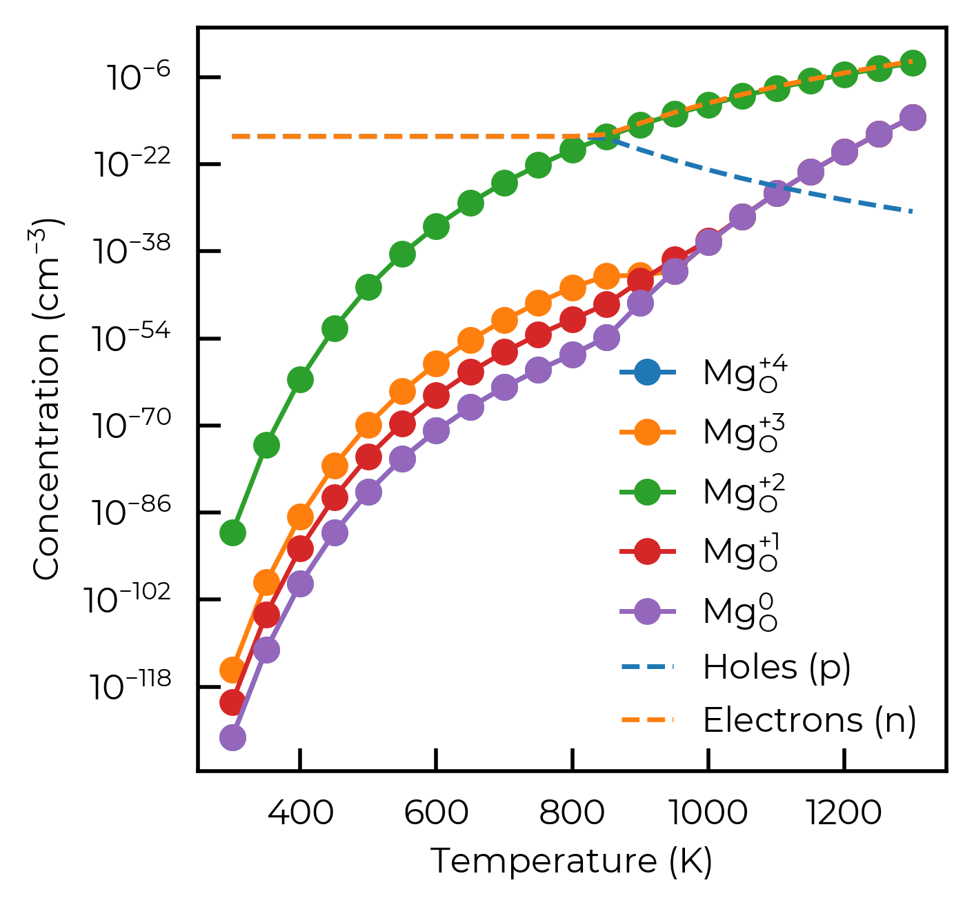
Because we have only included a single (very high formation energy) defect here, the Mg\(_O\) concentration is negligible and the carrier concentrations are essentially intrinsic (\(n \approx p\)) – again, this is just to illustrate the workflow.
For more thorough examples of defect thermodynamic analyses with doped – including self-consistent Fermi level determination, frozen (annealing/quenching) defect equilibria, effective doping limits, chemical potential scans, carrier concentration optimisation and more – see the thermodynamics analysis tutorial and the FermiSolver tutorial.
9.5 Analysing site displacements
We can check that our supercell is large enough by plotting the site displacements as a function of the site distance to the defect. The site displacements are calculated by comparing to the original position of the site in the pristine supercell.
If the supercell is large enough, the displacements should decay to zero as the distance from the defect increases.
from doped.utils.plotting import format_defect_name

plt.clf()
for defect_name, defect_entry in dp.defect_dict.items():
    formatted_defect_name = format_defect_name(defect_name, include_site_info=False)  # format name for plot title
    fig = defect_entry.plot_site_displacements(separated_by_direction=True)
    # Add title to figure with defect name, avoid overlap with subfigure titles
    fig.suptitle(formatted_defect_name, y=1.15)
plt.show()
<Figure size 1400x1400 with 0 Axes>
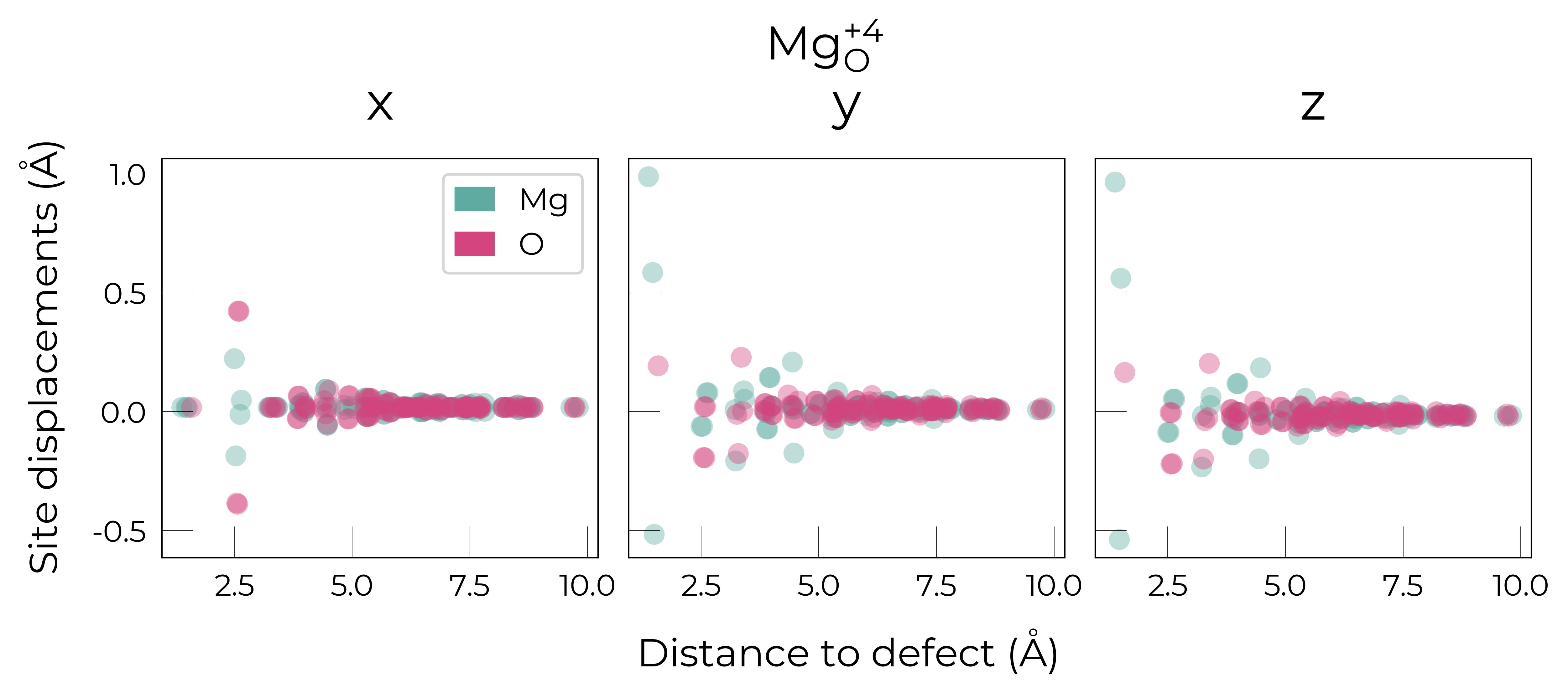
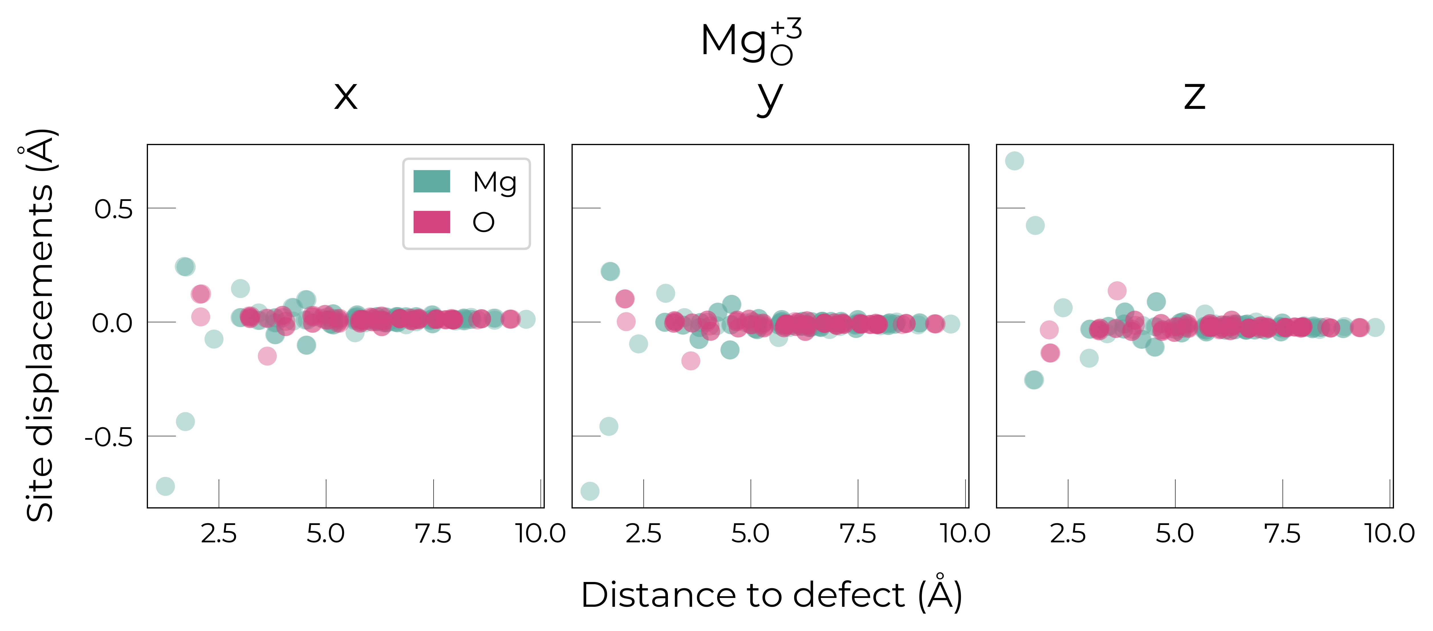
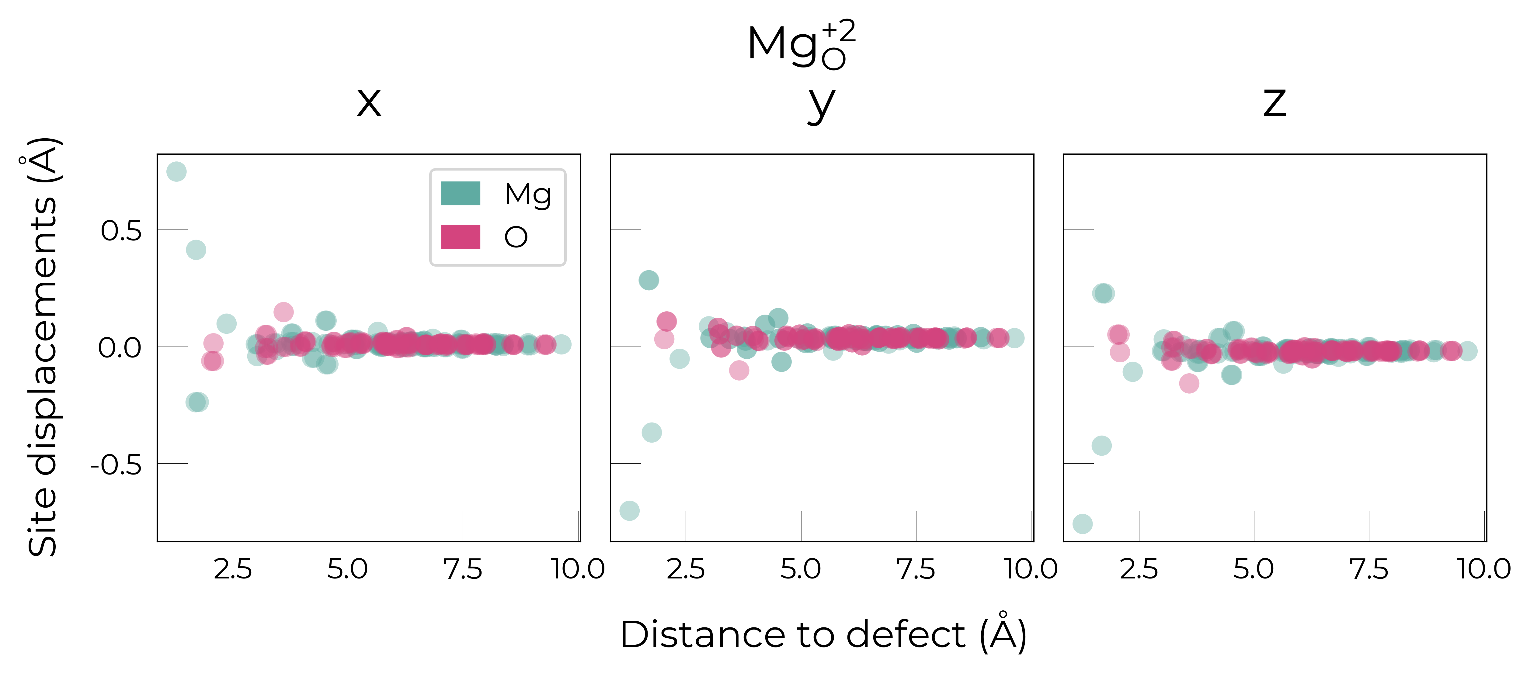
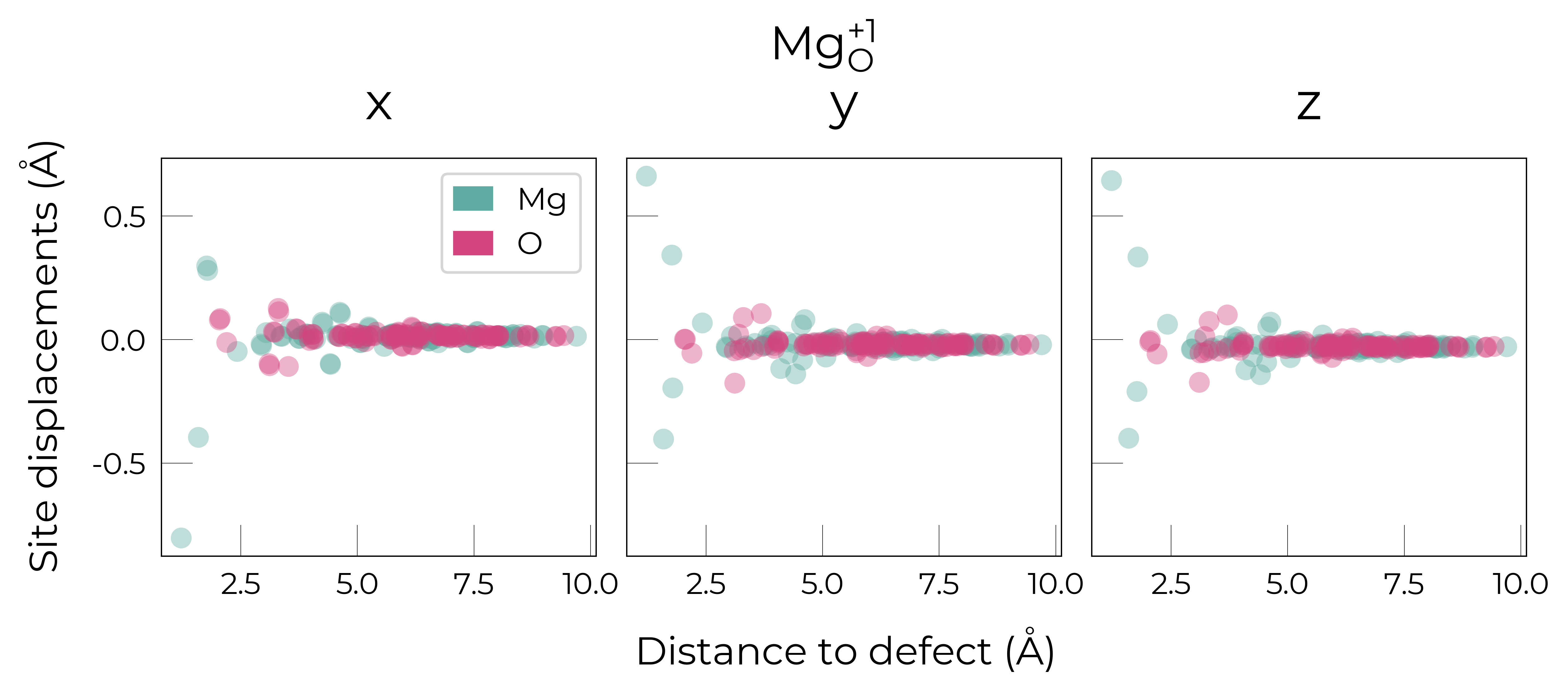
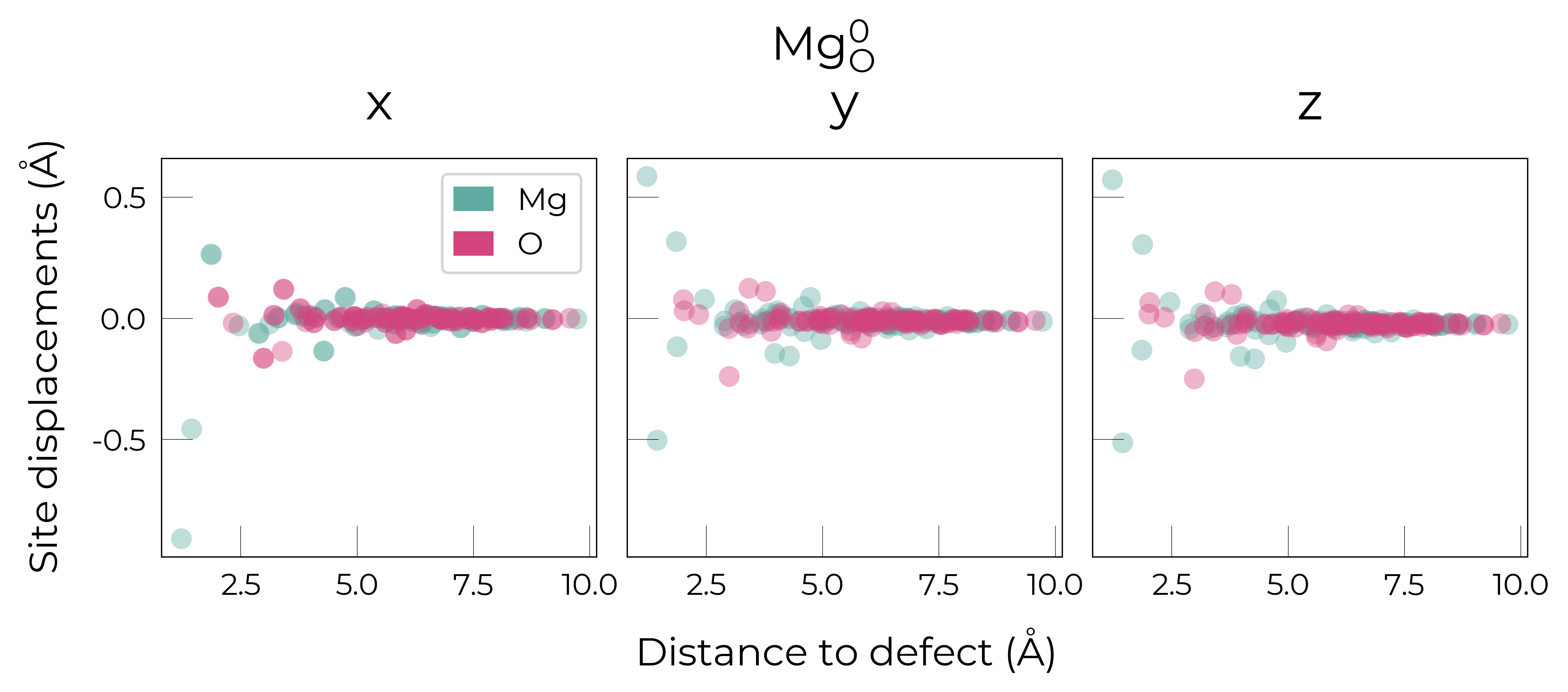
Let’s plot the displacements relative to the defect site instead:
from doped.utils.plotting import format_defect_name

plt.clf()
for defect_name, defect_entry in dp.defect_dict.items():
    formatted_defect_name = format_defect_name(defect_name, include_site_info=False)  # format name for plot title
    fig = defect_entry.plot_site_displacements()
    # Add title to figure with defect name, avoid overlap with subfigure titles
    fig.suptitle(formatted_defect_name)
plt.show()
<Figure size 2820x2760 with 0 Axes>
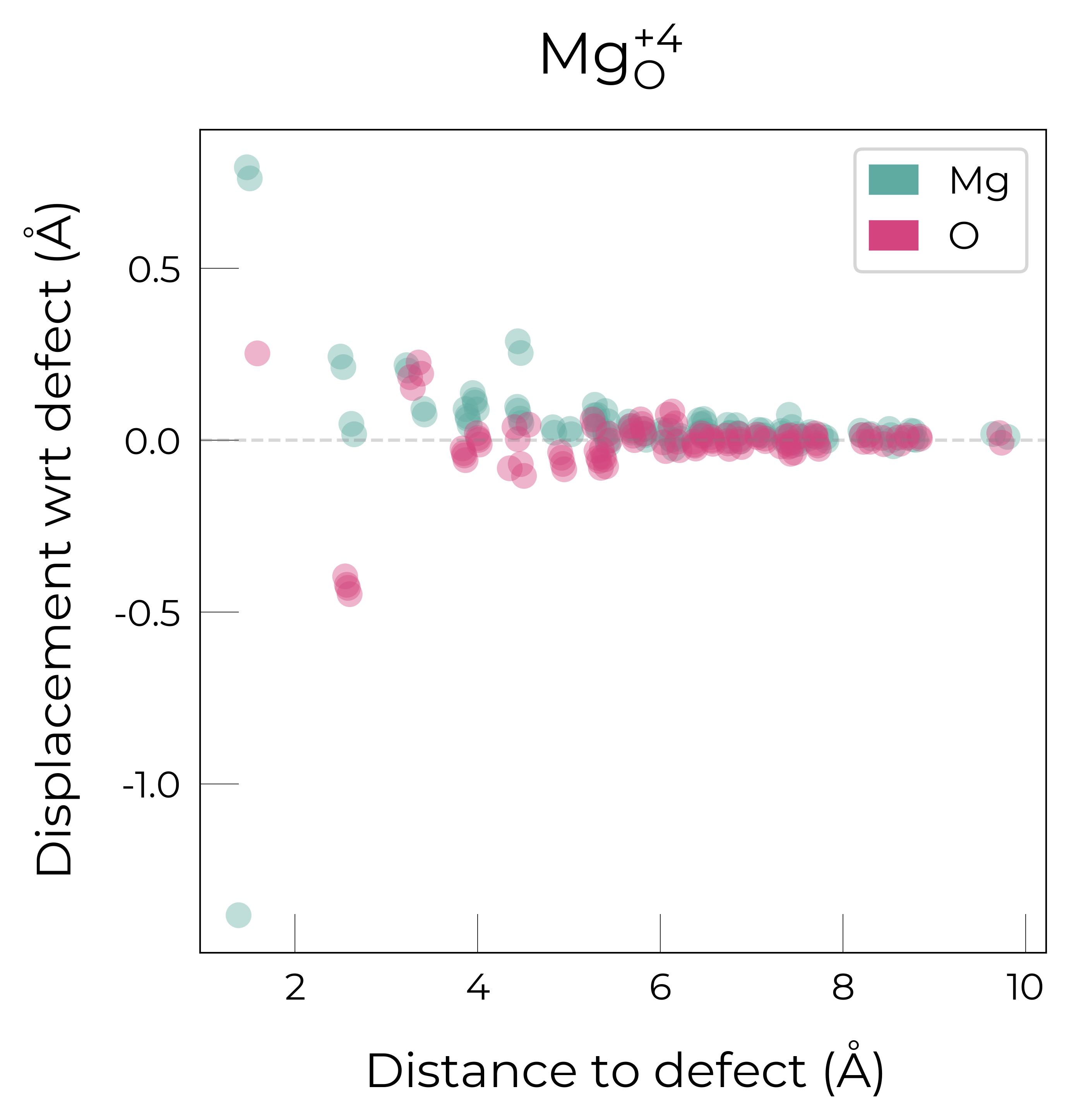
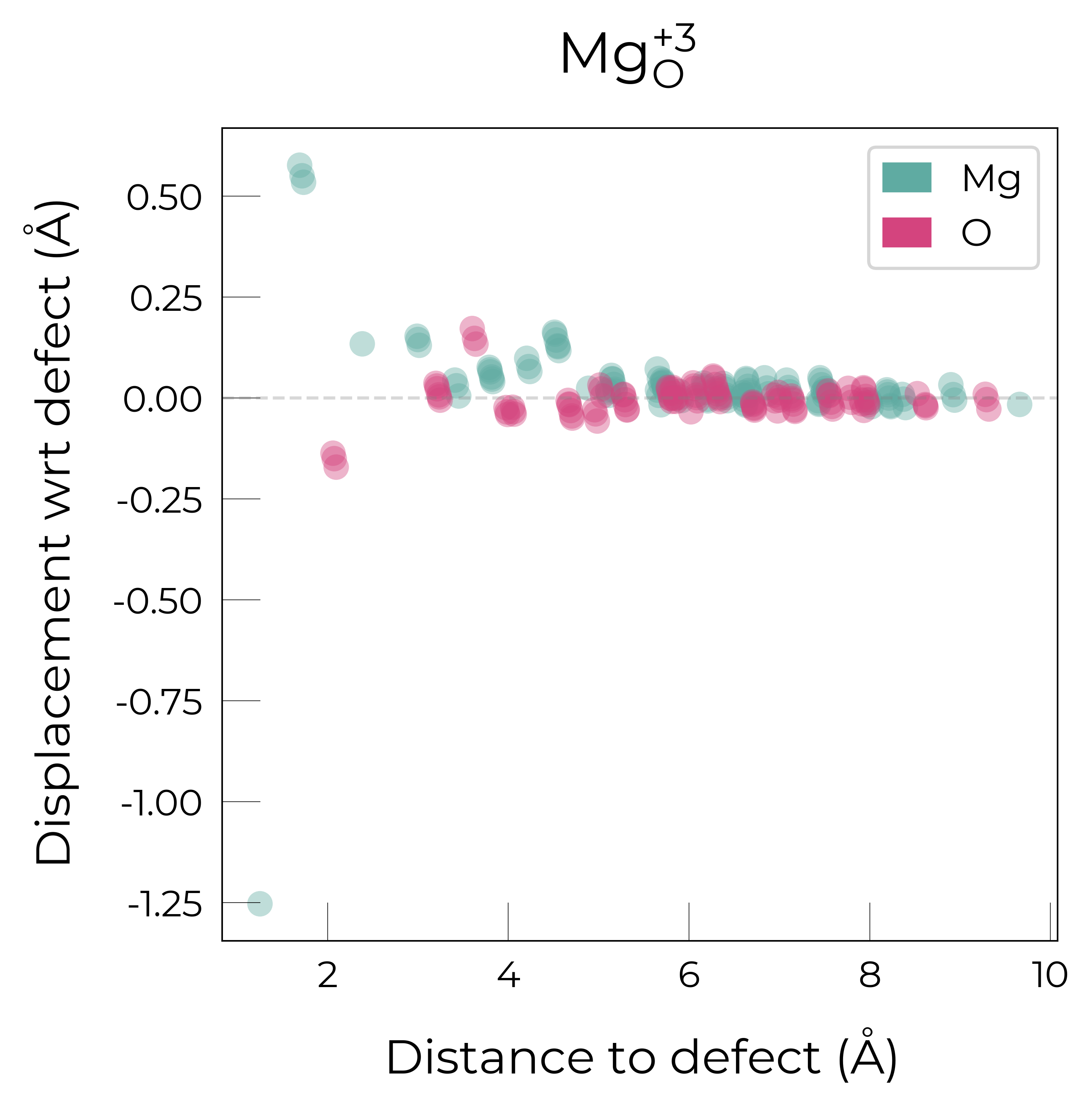
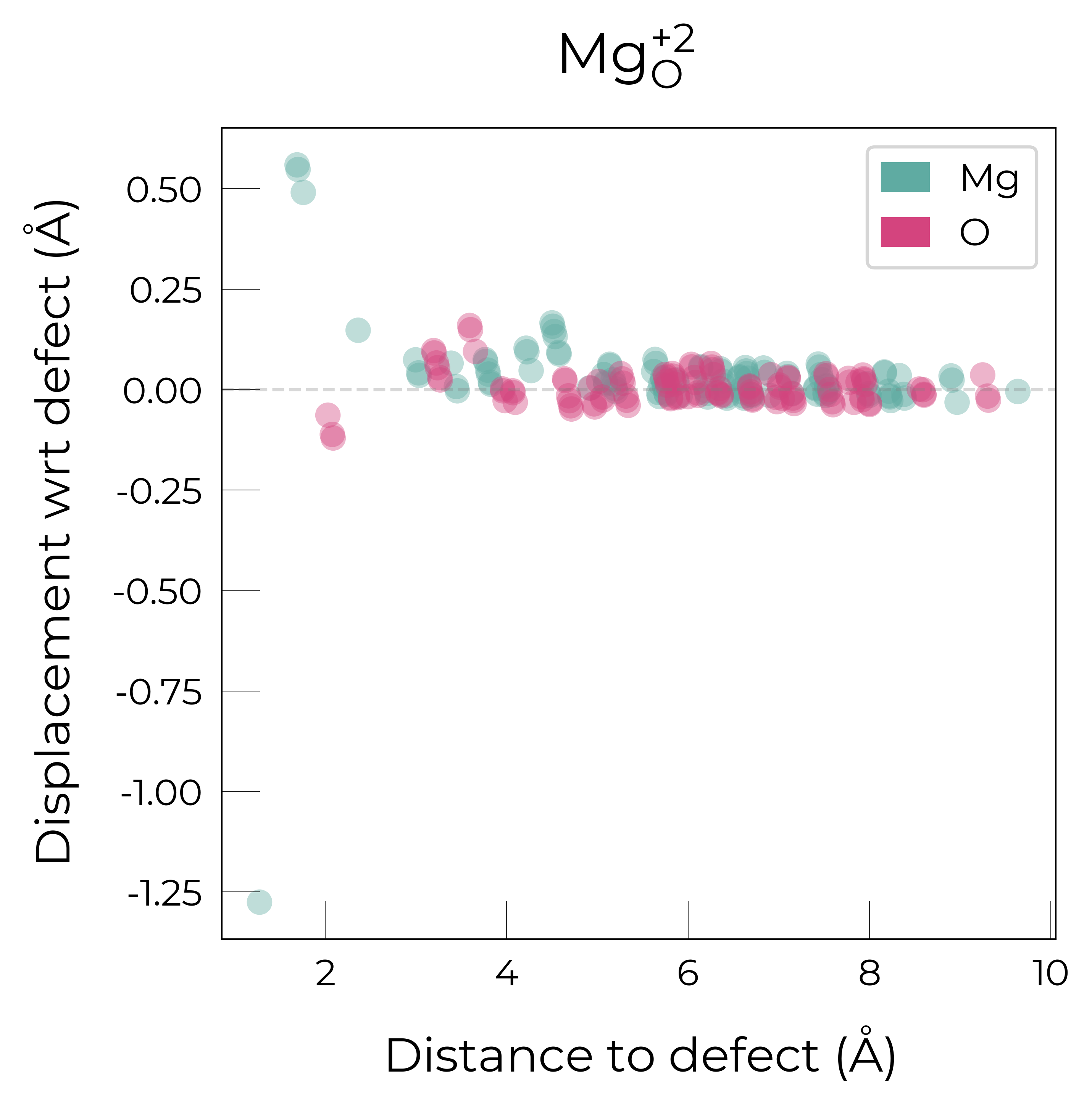
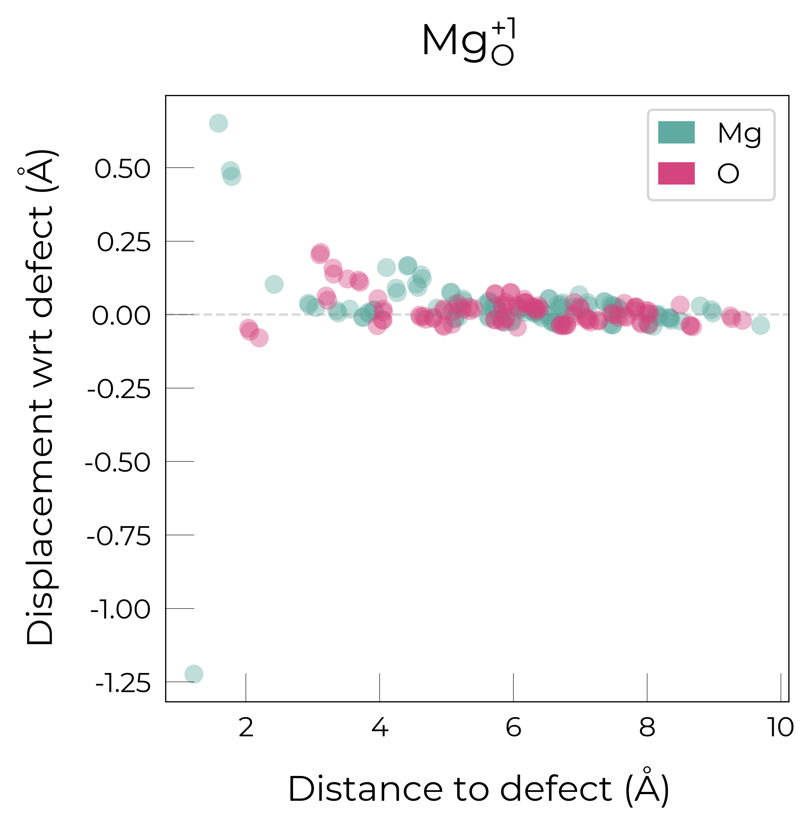
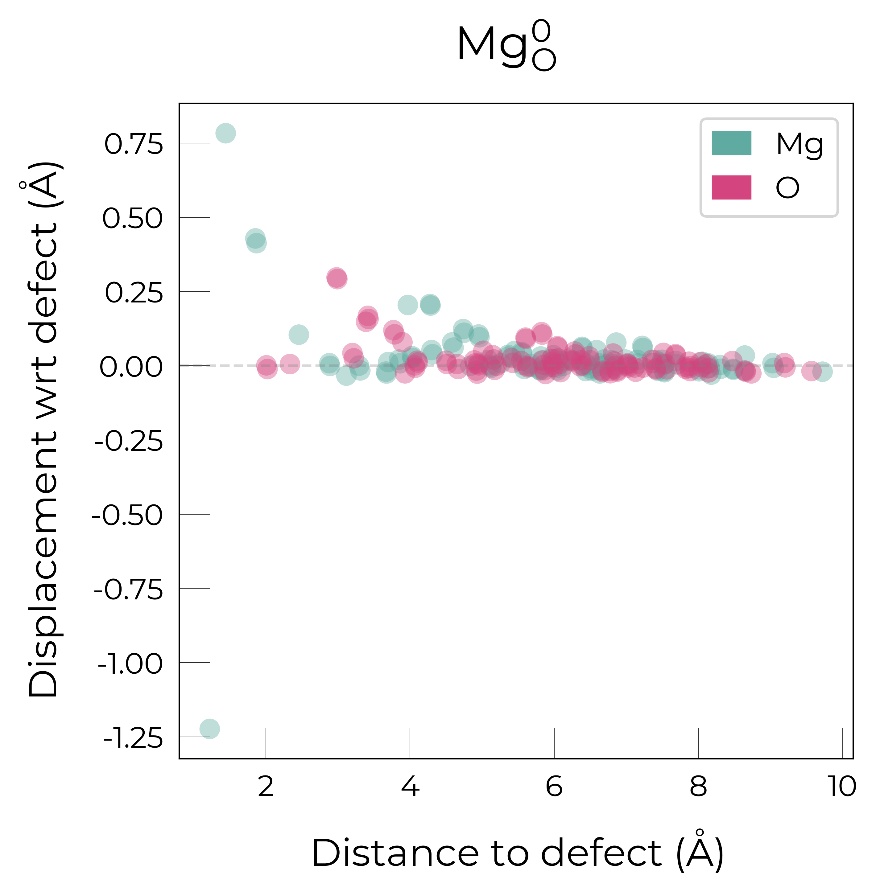
These displacement plots clearly show how the defect perturbation of the host structure tails off as we move away from the defect site. This is important for ensuring that the defect supercell is large enough.
In addition, we can also plot the site displacements relative to the defect. This can be useful to visualise which atoms move closer / further away from the defect (e.g. cases the 1st NN shell of the defect compresses (negative displacement) but 2nd NN expands (positve displacement)):
from monty.serialization import loadfn

# Loading defect dictionary from json
MgO_defect_dict = loadfn("MgO/MgO_defect_dict.json.gz")
defect_entry = MgO_defect_dict['Mg_O_0']  # Neutral defect
fig = defect_entry.plot_site_displacements(
    relative_to_defect=True,
)
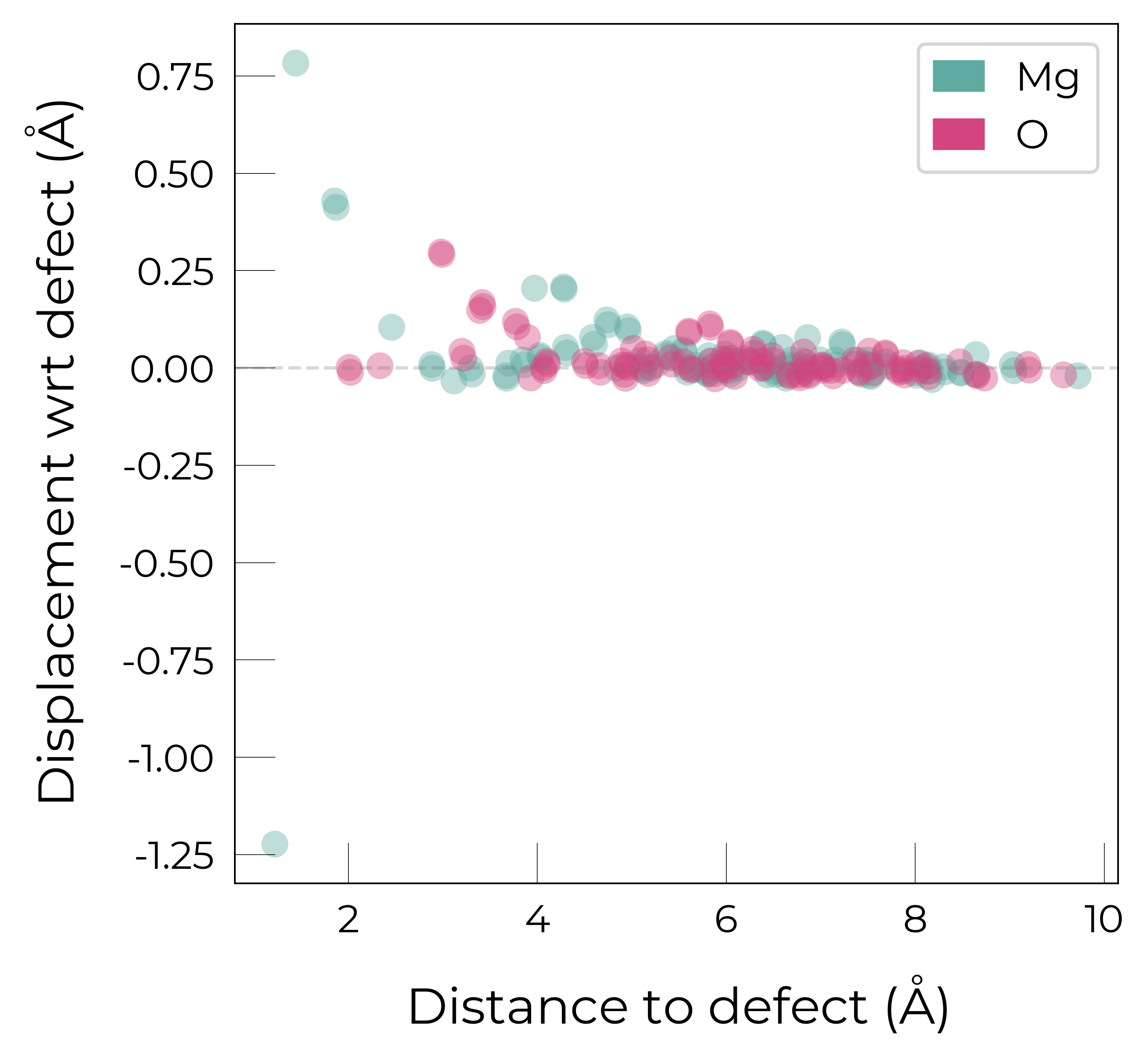
Which shows that the 3 Mg atoms in the 1st NN shell of the Mg antisite defect are displaced away the defect.
You can also project the displacements along a specified vector using the option vector_to_project_on:
fig = defect_entry.plot_site_displacements(
    vector_to_project_on=(0, 0, 1),  # Project on z-axis
)
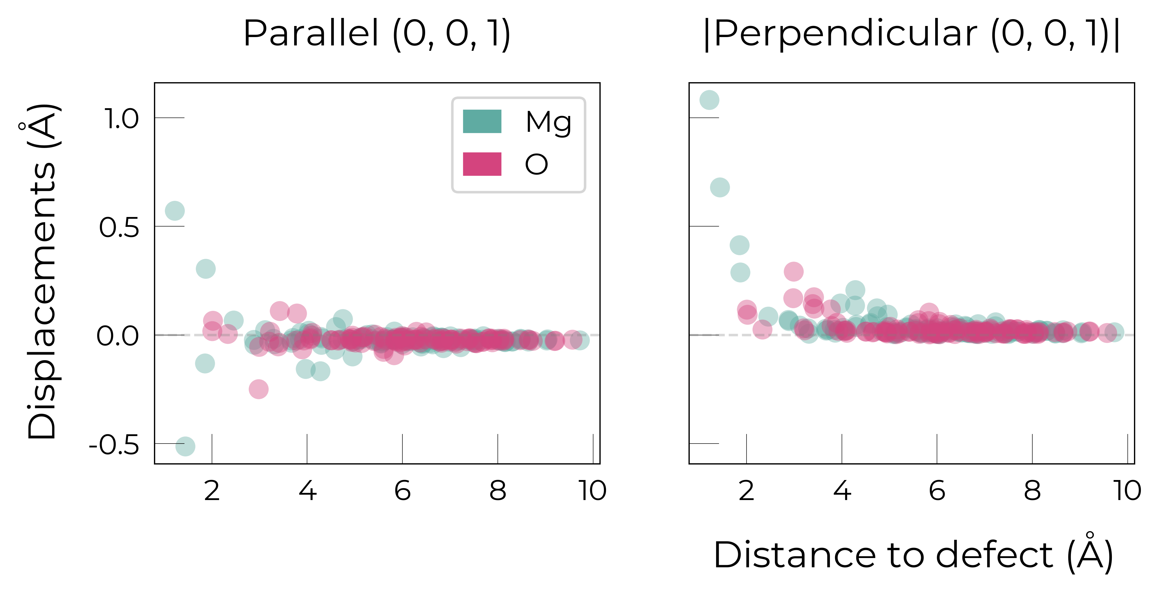
9.6 Analysing Finite-Size Charge Corrections
Kumagai-Oba (eFNV) Charge Correction Example:
As mentioned above, doped can automatically compute either the Kumagai-Oba (eFNV) or Freysoldt (FNV)
finite-size charge corrections, to account for the spurious image charge interactions in the defect
supercell approach (see the
YouTube/B站
defect tutorial for more details).
The eFNV correction is used by default if possible (if the required OUTCAR(.gz) files are available),
as it is more general – can be used for both isotropic and
anisotropic systems – and the numerical implementation is more efficient, requiring smaller file sizes
and running quicker.
Below, we show how to directly visualising the charge correction plots (showing how they are computed), which is recommended if any warnings about the charge correction accuracy are printed when parsing our defects (also useful for understanding how the corrections are performed!).
dp.defect_dict.keys()
dict_keys(['Mg_O_+4', 'Mg_O_+3', 'Mg_O_+2', 'Mg_O_+1', 'Mg_O_0'])
from doped.analysis import DefectParser  # can use DefectParser to parse individual defects if desired

defect_entry = dp.defect_dict["Mg_O_+4"]
print(f"Charge: {defect_entry.charge_state:+} at site: {defect_entry.defect_supercell_site.frac_coords}")
print(f"Finite-size charge corrections: {defect_entry.corrections}")
Charge: +4 at site: [0.50148977 0.57845999 0.57665118]
Finite-size charge corrections: {'kumagai_charge_correction': np.float64(2.5859785129575688)}
Above, the defect has been parsed and the anisotropic (eFNV) charge correction correctly applied, with no warnings thrown. We can directly plot the atomic site potentials which are used to compute this charge correction if we want: (Though typically we only do this if there has been some warning or error related to the application of the defect charge correction – here we’re just showing as a demonstration)
Note
Typically we only analyze the charge correction plots like this if there has been some warning or error related to the defect charge correction (or to aid our understanding of the underlying formation energy calculations). Here we’re just showing as a demonstration.
correction, plot = defect_entry.get_kumagai_correction(plot=True)
Calculated Kumagai (eFNV) correction is 2.586 eV
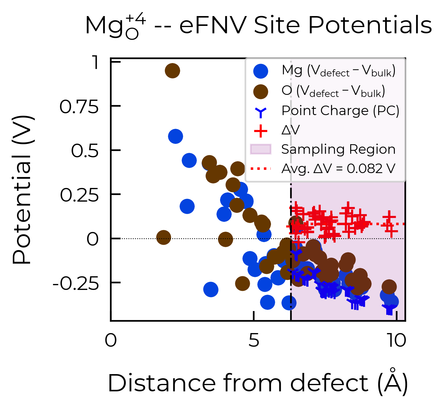
Here we can see we obtain a good plateau in the atomic potential differences (ΔV) between the defect and bulk supercells in the ‘sampling region’ (i.e. region of defect supercell furthest from the defect site), the average of which is used to obtain our potential alignment (‘Avg. ΔV’) and thus our final charge correction term.
If there is still significant variance in the site potential differences in the sampling region (i.e. a
converged plateau is not obtained), then this suggests that the charge correction may not be as accurate
for that particular defect or supercell. This error range of the charge correction is automatically
computed by doped, and can be returned using the return_correction_error argument in
get_kumagai_correction/get_freysoldt_correction, or also by adjusting the error_tolerance argument:
correction, error = defect_entry.get_kumagai_correction(return_correction_error=True)
error  # calculated error range of 18.2 meV in our charge correction here
Calculated Kumagai (eFNV) correction is 2.586 eV
np.float64(0.018215609608677574)
print(f"Relative error: {100*0.018215 / 2.586:.3f}%")
Relative error: 0.704%
which is a small error! ✅
9.7 Further Defect Analysis
As briefly discussed in the
YouTube/B站
defects tutorial, you will likely
want to further analyse the key defect species in your material, by e.g. visualising the relaxed
structures with VESTA/CrystalMaker, looking at the defect single-particle energy levels using the
sumo DOS plotting functions (sumo-dosplot), charge density
distributions (e.g. this Figure).
In particular, you may want to further analyse the behaviour and impact on material properties of your
defects using advanced defect analysis codes such as py-sc-fermi (to analyse defect concentrations, doping and Fermi level tuning), easyunfold (to analyse the electronic structure of defects in your
material), or nonrad / CarrierCapture.py (to analyse non-radiative electron-hole recombination at defects – for which the Configuration Coordinate Diagram Generation tutorial would likely be useful).
The outputs from doped are readily ported as inputs to these codes.
# folder cleanup for GitHub example files:
!rm -r MgO/SnB/Mg_O_* CompetingPhases/Mg_* CompetingPhases/MgO_* CompetingPhases/O2_* MgO/Defects/Mg* MgO/Bulk_DOS
zsh:1: no matches found: MgO/SnB/Mg_O_*