Advanced Defect/Carrier Concentration Analysis
Tip
You can run this notebook interactively through Google Colab or Binder – just click the links! (Then uncomment the !pip install... cell).
For advanced analysis of defect/carrier thermodynamics in doped, we provide the FermiSolver class. This class includes several key features, focusing on easy scanning of defect populations over multiple parameters of interest, such as temperature, chemical potential, “effective” external dopant concentrations, variable defect mobilities/constraints and more. Some particular points of interest are:
Methods for automatically scanning over a range of given parameters.
Interpolation between arbitrary points in chemical potential space for generating “Brouwer-like” diagrams.
Searching and mapping defect concentrations over the full chemical potential stability limits of a material.
Integration with py-sc-fermi allows for customising concentration constraints for subsets of defects, which can be particularly useful for considering systems where some, but not all, point defects are mobile.
There are two FermiSolver backends: doped and py-sc-fermi. Both provide similar functionality, but the py-sc-fermi backend extends what is possible with doped through an interface with the py_sc_fermi code. This includes some advanced analysis functionality, which we will describe in this notebook. Unless the user specifies which backend they would like, the code will default to doped and use py-sc-fermi when required.
CdTe: Defect Concentrations
We’ll start by using the familiar binary CdTe example to outline the basic functionality of the FermiSolver. Here we will showcase the functionality of FermiSolver by creating two instances with the different backends – of course you will likely only need to use one in your research.
# # If running on Colab; uncomment to install doped, clone the repo to download the example data and cd in to examples folder:
# !pip install doped
# !git clone https://github.com/SMTG-Bham/doped
# %cd doped/examples
In the simplest case, we can initialise FermiSolver directly from a DefectThermodynamics object (see the thermodynamics tutorial), using the already-set bulk_dos, chempots and el_refs parameters:
from doped.thermodynamics import FermiSolver
from monty.serialization import loadfn

defect_thermo = loadfn("CdTe/CdTe_LZ_thermo_wout_meta.json.gz")
fs = FermiSolver(defect_thermo)  # doped backend by default
However we can also add or overwrite the bulk DOS and chemical potentials data:
# we need to specify the path to the vasprun.xml(.gz) file
# that was used for the DOS calculation. This is because
# we need to accurately account for the electronic carrier concentrations
# as well as the defect concentrations to determine the Fermi level
vasprun_path = "CdTe/CdTe_prim_k181818_NKRED_2_vasprun.xml.gz"
# note that if we have already loaded our bulk DOS (``bulk_dos``) into the
# DefectThermodynamics object (e.g. with ``get_equilibrium_fermi_level``)
# we don't need to specify and re-parse ``bulk_dos`` below

# the DefectThermodynamics object contains all the information about the
# defect formation energies, degeneracy factors and transition levels.
# It will underpin both the doped and py-sc-fermi solvers
defect_thermo = loadfn("CdTe/CdTe_LZ_thermo_wout_meta.json.gz")

# and the chemical potentials can then be used to specify the
# defect formation energies under different conditions, and act as a parameter
# space we can scan over to interrogate the defect concentrations
chempots = loadfn("CdTe/CdTe_chempots.json")

# initialize the FermiSolver objects. These require information about the
# defect thermodynamics and the electronic structure of the bulk material. The
# chempots argument can be supplied to overwrite any chempots associated with
# the defect thermodynamics object, but regardless chempots must be supplied
fs = FermiSolver(
    defect_thermodynamics=defect_thermo, bulk_dos=vasprun_path, chempots=chempots, backend="doped"
)  # default backend
py_fs = FermiSolver(
    defect_thermodynamics=defect_thermo, bulk_dos=vasprun_path, chempots=chempots, backend="py-sc-fermi"
)
Once we have the FermiSolvers, perhaps the simplest parameter to scan over is the temperature, and we can do so as follows. We will use this as an example to show that the two solvers return the same results for the same input data.
# define a range of temperatures to scan over
import pandas as pd

temperatures = range(300, 1410, 50)  # temperatures to consider, in K
# the scan_temperature method can be used to scan over a range of temperatures
# and generate a DataFrame containing the defect concentrations, carrier concentrations,
# and Fermi levels at each temperature. We can specify the chemical potentials as
# a limit,
temperature_df = fs.scan_temperature(limit="Cd-rich", temperature_range=temperatures)

# or they can be specified as a dictionary of chemical potentials referenced to the
# elements in the bulk structure
temperature_df_py = py_fs.scan_temperature(  # manually specify Cd-rich chempots
    chempots={"Cd": 0.0, "Te": -1.2513}, temperature_range=temperatures
)
100%|██████████| 23/23 [00:00<00:00, 57.81it/s]
100%|██████████| 23/23 [00:01<00:00, 22.49it/s]
# this outputs a dataframe of our defect & carrier concentrations at each temperature and chemical potential:
temperature_df.tail()
| Concentration (cm^-3) | Temperature (K) | Fermi Level (eV wrt VBM) | Electrons (cm^-3) | Holes (cm^-3) | μ_Cd (eV) | μ_Te (eV) | |
|---|---|---|---|---|---|---|---|
| Defect | |||||||
| Te_Cd | 4.151297e+08 | 1400.0 | 1.10229 | 2.336290e+17 | 2.168583e+16 | 0.0 | -1.251317 |
| Cd_i_Td_Cd2.83 | 8.359981e+15 | 1400.0 | 1.10229 | 2.336290e+17 | 2.168583e+16 | 0.0 | -1.251317 |
| Cd_i_Td_Te2.83 | 9.655787e+16 | 1400.0 | 1.10229 | 2.336290e+17 | 2.168583e+16 | 0.0 | -1.251317 |
| Te_i_Td_Te2.83_a | 1.198971e+12 | 1400.0 | 1.10229 | 2.336290e+17 | 2.168583e+16 | 0.0 | -1.251317 |
| Te_i_Td_Te2.83_b | 1.067428e+06 | 1400.0 | 1.10229 | 2.336290e+17 | 2.168583e+16 | 0.0 | -1.251317 |
Let’s plot the results:
import matplotlib.pyplot as plt
import doped

# we can use the doped style file to make all our plots look consistent
plt.style.use(f"{doped.__path__[0]}/utils/doped.mplstyle")  # use doped style
from doped.utils.plotting import format_defect_name
# we can specify the colors to use for each defect, so that the same defect
# is plotted in the same color for both backends, and we keep all our plots consistent
defect_colors = {
    "Te_Cd": "C0",
    "Cd_Te": "C1",
    "v_Cd": "C2",
    "v_Te": "C3",
    "Cd_i_Td_Cd2.83": "C4",
    "Cd_i_Td_Te2.83": "C5",
    "Te_i_Td_Te2.83_a": "C6",
    "Te_i_Td_Te2.83_b": "C7",
}

# label the results with the backend used to generate them, and concatenate the results
temperature_df["backend"] = "doped"
temperature_df_py["backend"] = "py-sc-fermi"
plot_data = pd.concat([temperature_df, temperature_df_py])

# Create a unique list of defects in the DataFrame
unique_defects = temperature_df.index.unique()

fig, ax = plt.subplots()

# loop over the unique defects and plot the defect concentrations
# as a function of temperature, for both the doped and py-sc-fermi backends
for defect in unique_defects:
    defect_df = plot_data.loc[defect]

    for backend in ["doped", "py-sc-fermi"]:
        defect_df_backend = defect_df[defect_df["backend"] == backend]
        ax.plot(
            defect_df_backend["Temperature (K)"],
            defect_df_backend["Concentration (cm^-3)"],
            label=format_defect_name(defect, include_site_info=True, wout_charge=True),
            color=defect_colors[defect],
            marker="o" if backend == "doped" else "x",
            alpha=0.25,
        )

ax.set_xlabel("Temperature (K)")
ax.set_ylabel("Concentration (cm$^{-3}$)")

ax.set_xlim(300, 1400)
ax.set_ylim(1e13, 1e18)
ax.set_yscale("log")

custom_lines = [plt.Line2D([0], [0], color=defect_colors[defect], lw=1) for defect in unique_defects]
custom_lines.append(plt.Line2D([0], [0], color="black", lw=1, marker="o", linestyle="None", label="doped"))
custom_lines.append(plt.Line2D([0], [0], color="black", lw=1, marker="x", linestyle="None", label="py-sc-fermi"))
ax.legend(custom_lines,
          [f"{format_defect_name(defect, include_site_info_in_name=True, wout_charge=True)}" for defect in unique_defects] + ["doped", "py-sc-fermi"],
          frameon=False)

plt.show()
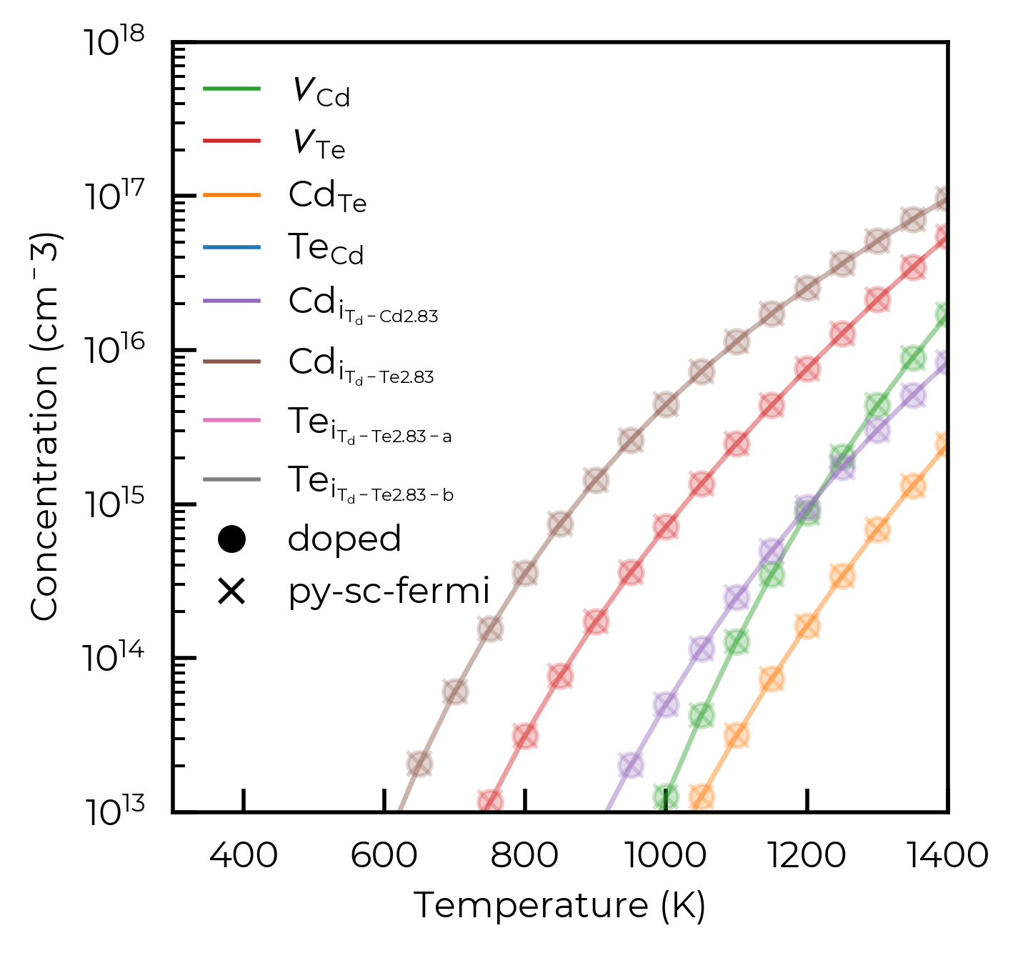
From the plot above, it is clear that when scanning the temperature, the defect concentrations reported by the two back-ends are essentially identical.
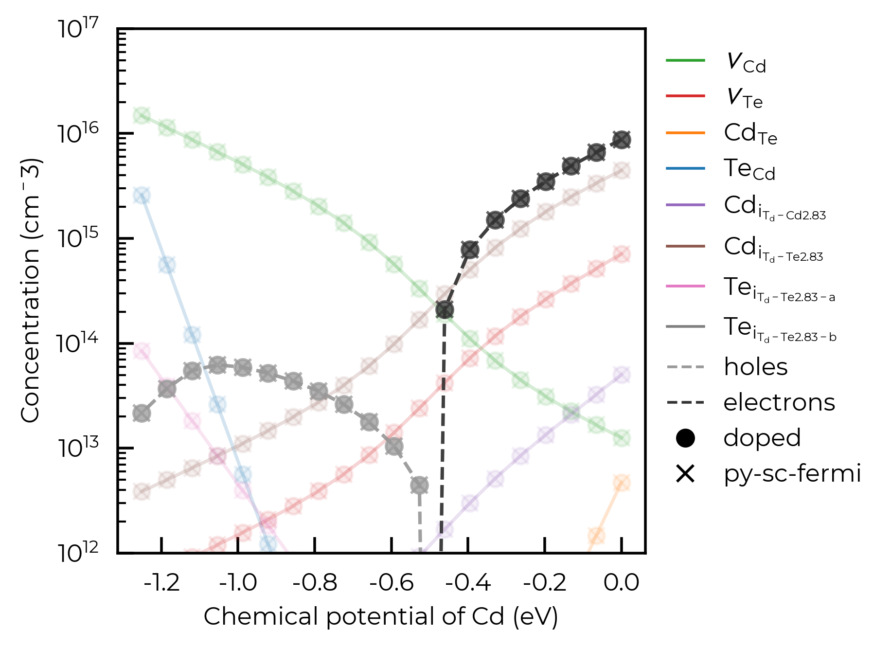
To continue to show the functionality of the FermiSolver, we’ll show how we can generate a Brouwer-digaram-like figure, with defect concentrations shown as a function of chemical potentials.
These scanning methods (including scan_temperature) can accept annealing_temperatures and quenched_temperatures arguments instead of temperature. These will carry out “frozen-defect” calculations between these temperatures as discussed in the defect thermodynamics tutorial.
In this cell, we’ll continue to directly compare the results of py-sc-fermi and doped.
# scan between the Cd and Te rich limits to see how the defect concentrations
# change as a function of chemical potential
mu_df = py_fs.interpolate_chempots(
    limits=["Cd-rich", "Te-rich"], n_points=20, annealing_temperature=1000, quenched_temperature=300
)
mu_df_doped = fs.interpolate_chempots(
    limits=["Cd-rich", "Te-rich"], n_points=20, annealing_temperature=1000, quenched_temperature=300
)

# we'll keep the py-sc-fermi and doped comparison going, especially as we have made
# the solution slightly more complex by introducing the annealing-quenching process.
mu_df["backend"] = "py-sc-fermi"
mu_df_doped["backend"] = "doped"
mu_df = pd.concat([mu_df, mu_df_doped])

fig, ax = plt.subplots()

# loop over the unique defects and plot their defect concentrations as a function
# of the chemical potential of Cd, for both the doped and py-sc-fermi backends
for backend in ["py-sc-fermi", "doped"]:
    for defect in unique_defects:
        defect_df = mu_df.loc[defect]
        defect_df_backend = defect_df[defect_df["backend"] == backend]
        ax.plot(
            defect_df_backend["μ_Cd (eV)"],
            defect_df_backend["Concentration (cm^-3)"],
            label=format_defect_name(defect, include_site_info=True, wout_charge=True),
            color=defect_colors[defect],
            marker="o" if backend == "doped" else "x",
            alpha=0.1,
        )
    ax.plot(
        defect_df_backend["μ_Cd (eV)"],
        defect_df_backend["Holes (cm^-3)"],
        marker="o" if backend == "doped" else "x",
        linestyle="--",
        alpha=0.75,
        color="#999999",
    )
    ax.plot(
        defect_df_backend["μ_Cd (eV)"],
        defect_df_backend["Electrons (cm^-3)"],
        marker="o" if backend == "doped" else "x",
        linestyle="--",
        alpha=0.75,
        color="#333333",
    )

ax.set_xlabel("Chemical potential of Cd (eV)")
ax.set_ylabel("Concentration (cm$^{-3}$)")

# legend formatting
custom_lines = [plt.Line2D([0], [0], color=defect_colors[defect], lw=1) for defect in unique_defects]
custom_lines.append(plt.Line2D([0], [0], color="#999999", lw=1, linestyle="--", label="holes"))
custom_lines.append(plt.Line2D([0], [0], color="#333333", lw=1, linestyle="--", label="electrons"))
custom_lines.append(plt.Line2D([0], [0], color="black", lw=1, marker="o", linestyle="None", label="doped"))
custom_lines.append(plt.Line2D([0], [0], color="black", lw=1, marker="x", linestyle="None", label="py-sc-fermi"))
plt.legend(custom_lines,
          [f"{format_defect_name(defect, include_site_info_in_name=True, wout_charge=True)}" for defect in unique_defects] + ["holes", "electrons", "doped", "py-sc-fermi"],
          frameon=False, loc="upper left", bbox_to_anchor=(1, 1))
plt.ylim(1e12, 1e17)
plt.yscale("log")
plt.show()
100%|██████████| 20/20 [00:00<00:00, 25.06it/s]
100%|██████████| 20/20 [00:01<00:00, 19.80it/s]
Tip
As always, see the code documentation for details on further customisation and control with these functions!
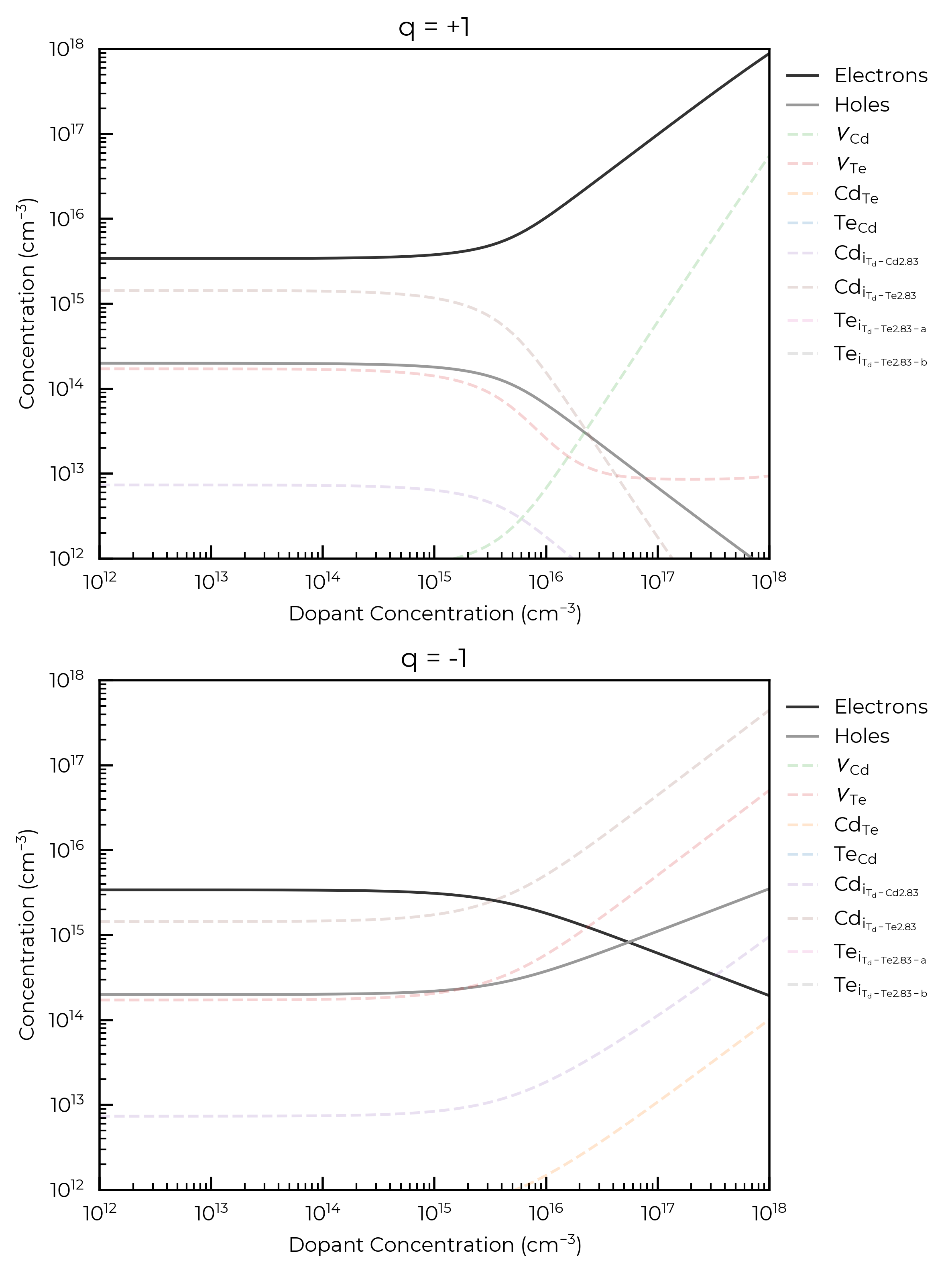
Effective dopant concentrations
In certain cases, we would like to directly simulate the effect of adding a dopant into our system to see how it will change the defect concentrations. If we treat the dopant concentration as an additional free parameter, we can change our charge neutrality condition from
to
where \(M\) is the concentration of the dopant with charge \(r\). As we are treating this as a free parameter, \(r[M^r]\) can be considered as single parameter, an effective dopant concentration that we can additionally scan over when investigating defect concentrations.
This analysis can be useful for investigating the host defect response to an as-yet-unidentified dopant/impurity; predicting how the Fermi level and defect/carrier concentrations will change in response to a range of possible dopant concentrations. Or in other words, for analysing the dopability and compensation response, which can be useful for investigating potential solar cell / transparent conductor / thermoelectric / battery materials and more.
See, for example:
This can be investigated in doped using the effective_dopant_concentration parameter in the Fermi level solving functions (both with DefectThermodynamics and the FermiSolver objects):
def plot_dopant_data(ax, df, concentrations, defect, color, **kwargs):
"""Simple function to handle the plotting in the following cells"""
defect_df = df.loc[defect]
ax.plot(
concentrations,
defect_df["Concentration (cm^-3)"],
label=format_defect_name(defect, include_site_info=True, wout_charge=True) or "Dopant",
color=color,
alpha=0.2,
**kwargs,
)
ax.set_xscale("log")
ax.set_yscale("log")
ax.set_xlabel("Dopant Concentration (cm$^{-3}$)")
ax.set_ylabel("Concentration (cm$^{-3}$)")
ax.legend(frameon=False, loc="upper left", bbox_to_anchor=(1, 1))
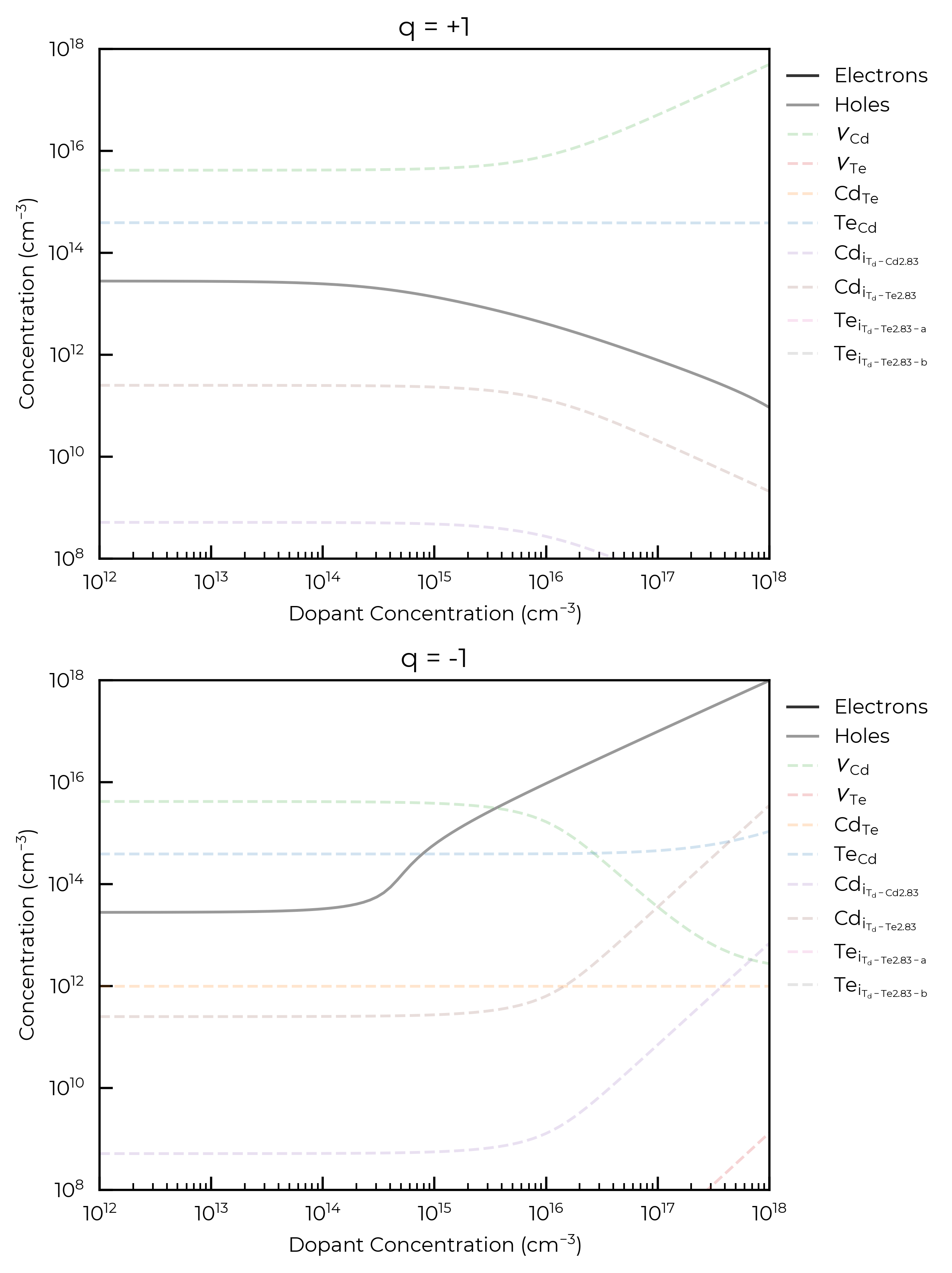
def plot_dopant_carrier_concentrations(dopant_df_positive, dopant_df_negative, ax):
ax[0].plot(dopant_df_positive["Dopant (cm^-3)"], dopant_df_positive["Electrons (cm^-3)"], label="Electrons", color="#333333")
ax[0].plot(dopant_df_positive["Dopant (cm^-3)"], dopant_df_positive["Holes (cm^-3)"], label="Holes", color="#999999")
ax[1].plot(-dopant_df_negative["Dopant (cm^-3)"], dopant_df_negative["Electrons (cm^-3)"], label="Electrons", color="#333333")
ax[1].plot(-dopant_df_negative["Dopant (cm^-3)"], dopant_df_negative["Holes (cm^-3)"], label="Holes", color="#999999")
# scan a positive and negative effective dopant concentration range - note this can
# be done with both the doped and py-sc-fermi backends. We will just use the doped backend
# for this example.
import numpy as np
dopant_concentrations = np.logspace(12, 18, 100)
defect_colors.update({"Dopant": "gray"})
dopant_df_positive = fs.scan_dopant_concentration(
chempots={"Cd": 0.0, "Te": -1.251},
temperature=900,
effective_dopant_concentration_range=dopant_concentrations,
)
dopant_df_negative = fs.scan_dopant_concentration(
chempots={"Cd": 0.0, "Te": -1.251},
temperature=900,
effective_dopant_concentration_range=-1 * dopant_concentrations,
)
fig, ax = plt.subplots(2, 1, figsize=(6, 8))
plot_dopant_carrier_concentrations(dopant_df_positive, dopant_df_negative, ax)
for defect in dopant_df_positive.index.unique():
plot_dopant_data(ax[0], dopant_df_positive, dopant_concentrations, defect, defect_colors[defect], ls="--")
plot_dopant_data(ax[1], dopant_df_negative, dopant_concentrations, defect, defect_colors[defect], ls="--")
ax[0].set_xlim(1e12, 1e18); ax[1].set_xlim(1e12, 1e18)
ax[0].set_ylim(1e12, 1e18); ax[1].set_ylim(1e12, 1e18)
ax[0].set_title(f"q = +1"); ax[1].set_title(f"q = -1")
plt.tight_layout()
plt.show()
100%|██████████| 100/100 [00:02<00:00, 45.24it/s]
100%|██████████| 100/100 [00:02<00:00, 44.16it/s]
The cell below illustrates the same functionality, but we now have an annealing and quenching temperature, this requires minimal changes to the code. The plot_data function from the cell above is used again:
dopant_concentrations = np.logspace(12, 18, 100)
fig, ax = plt.subplots(2, 1, figsize=(6, 8))

# the only difference here is that we're scanning over dopant concentration
# having annealed at 900 K and quenched to 300 K
dopant_df_positive = fs.scan_dopant_concentration(
    chempots=chempots["limits_wrt_el_refs"]["Cd-CdTe"],
    annealing_temperature=900,
    quenched_temperature=300,
    effective_dopant_concentration_range=dopant_concentrations,
)
dopant_df_negative = fs.scan_dopant_concentration(
    limit="Cd-rich",
    quenched_temperature=300,
    annealing_temperature=900,
    effective_dopant_concentration_range=-dopant_concentrations,
)

plot_dopant_carrier_concentrations(dopant_df_positive, dopant_df_negative, ax)
for defect in dopant_df_positive.index.unique():
    plot_dopant_data(ax[0], dopant_df_positive, dopant_concentrations, defect, defect_colors[defect], ls="--")
    plot_dopant_data(ax[1], dopant_df_negative, dopant_concentrations, defect, defect_colors[defect], ls="--")

ax[0].set_xlim(1e12, 1e18); ax[1].set_xlim(1e12, 1e18)
ax[0].set_ylim(1e12, 1e18); ax[1].set_ylim(1e12, 1e18)
ax[0].set_title(f"q = +1"); ax[1].set_title(f"q = -1")
plt.tight_layout()
plt.show()
100%|██████████| 100/100 [00:06<00:00, 14.59it/s]
100%|██████████| 100/100 [00:06<00:00, 14.74it/s]
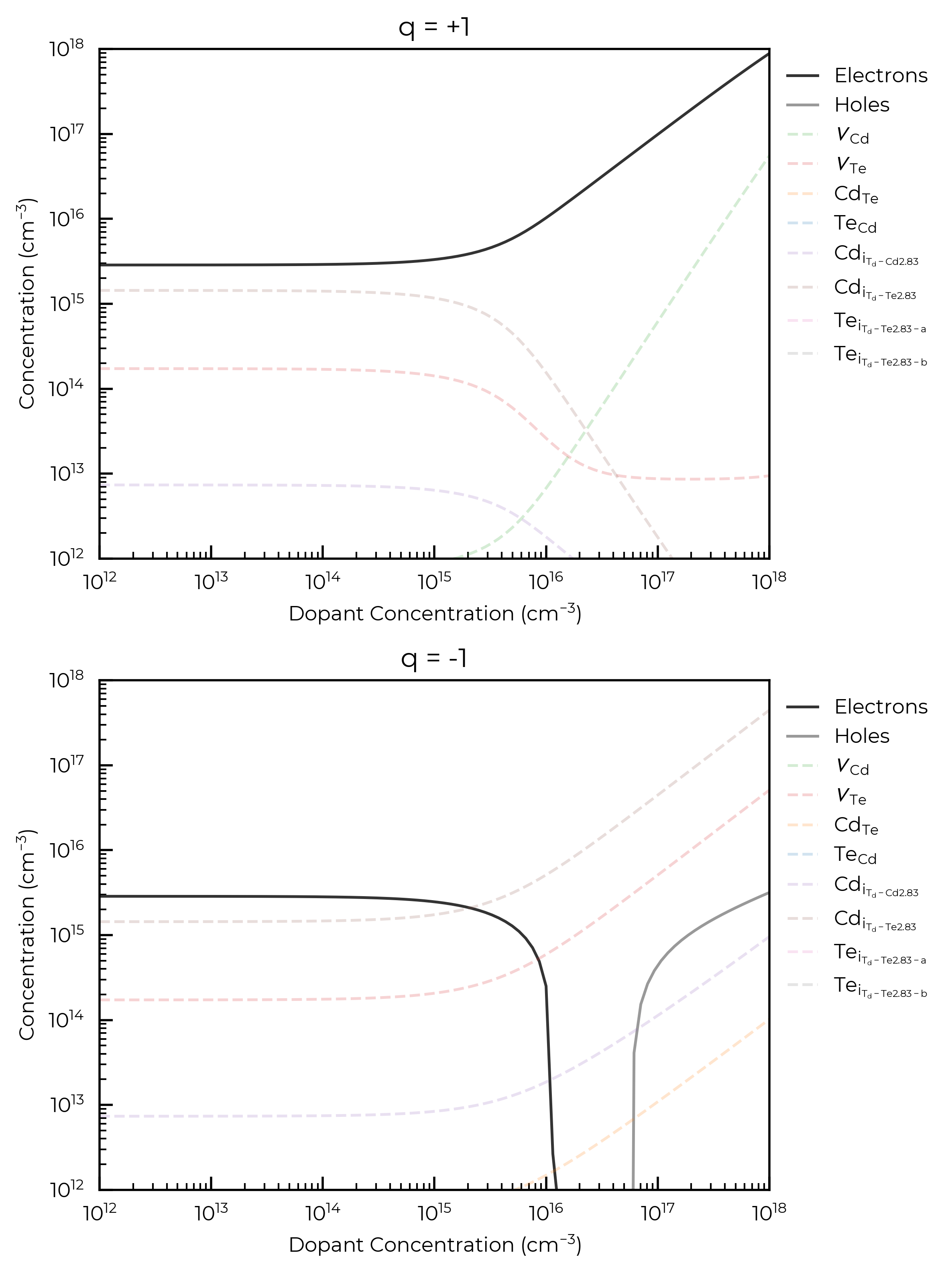
For both donor and acceptor dopants here, we see that a concentration \(>10^{15}\) cm\(^{-3}\) is required to significantly affect the Fermi level and thus carrier and intrinsic defect concentrations, for an annealing temperature of 900 K. This is the point at which the dopant concentration is equivalent to the concentrations of the highest-concentration intrinsic defects in the system and can be thought of as now influencing the Fermi energy “pinning”.
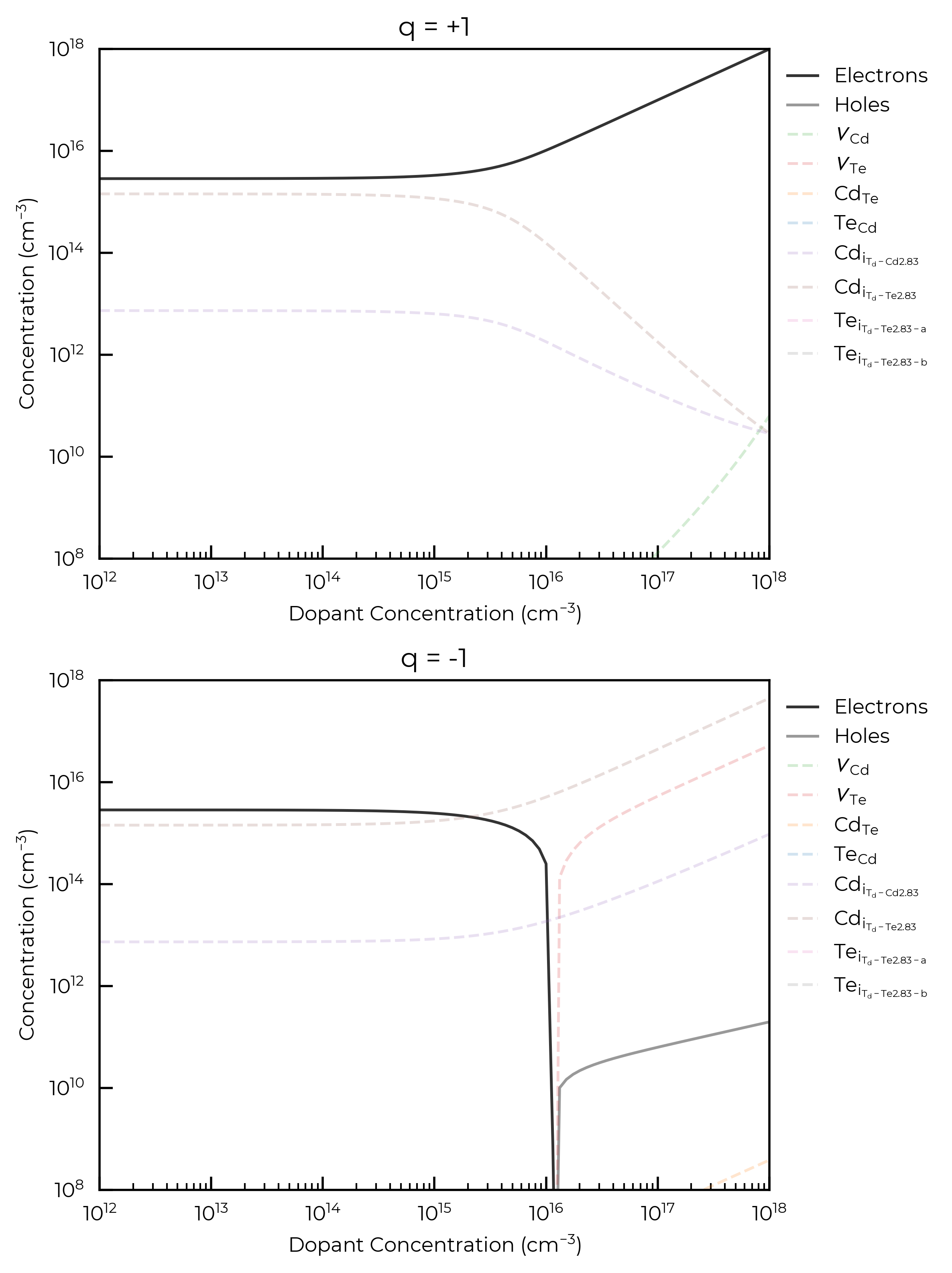
Custom Concentration/Equilibration Constraints
One thing we can do in py-sc-fermi is specify defects to be excluded from the ‘frozen defect’ approximation (i.e. the assumption that the total defect concentration will remain fixed at the high temperature value). This is useful in systems where we expect barriers for some defect recombination to be low. Take the example of an ion conductor, if interstitials of the mobile ion \(M\) form at high temperature, it may be unreasonable to assume these defects cannot then move into vacant \(M\) sites on cooling. For example, see
Squires et al., Low electronic conductivity of Li7La3Zr2O12 solid electrolytes from first principles
To explore these kinds of what if situations, all the quenching & annealing FermiSolver methods can accept an additional free-defects argument when using the "py-sc-fermi" backend, which specifies defects that are allowed to fully re-equilibrate at the quenched temperature (i.e. for which the ‘frozen defect’ approximation is not applied). The cell below shows this hypothetical example where the Te interstitials (known to be highly-mobile) and vacancies are allowed to recombine on cooling, but the total concentrations of all other defects remain fixed at the high temperature values (‘frozen defect’ approximation).
dopant_concentrations = np.logspace(12, 18, 100)
fig, ax = plt.subplots(2, 1, figsize=(6, 8))

dopant_df_positive = py_fs.scan_dopant_concentration(
    limit="Te-rich",
    annealing_temperature=900,
    quenched_temperature=300,
    effective_dopant_concentration_range=dopant_concentrations,
    free_defects=["Te_i_Td_Te2.83", "v_Te"],
)
dopant_df_negative = py_fs.scan_dopant_concentration(
    limit="Te-rich",
    annealing_temperature=900,
    quenched_temperature=300,
    effective_dopant_concentration_range=-dopant_concentrations,
    free_defects=["Te_i_Td_Te2.83", "v_Te"],
)

plot_dopant_carrier_concentrations(dopant_df_positive, dopant_df_negative, ax)
for defect in dopant_df_positive.index.unique():
    color = next(v for k, v in defect_colors.items() if k in defect)
    plot_dopant_data(ax[0], dopant_df_positive, dopant_concentrations, defect, color, ls="--")
    plot_dopant_data(ax[1], dopant_df_negative, dopant_concentrations, defect, color, ls="--")

ax[0].set_xlim(1e12, 1e18); ax[1].set_xlim(1e12, 1e18)
ax[0].set_ylim(1e8, 1e18); ax[1].set_ylim(1e8, 1e18)
ax[0].set_title(f"q = +1"); ax[1].set_title(f"q = -1")
plt.tight_layout()
plt.show()
100%|██████████| 100/100 [00:13<00:00,  7.32it/s]
100%|██████████| 100/100 [00:07<00:00, 13.04it/s]
As an additional, purely-illustrative example, the below code cell shows the case where vacancies and antisites are allowed to recombine upon cooling, while interstitials are kept fixed at their high temperature concentrations:
dopant_concentrations = np.logspace(12, 18, 100)
fig, ax = plt.subplots(2, 1, figsize=(6, 8))

dopant_df_positive = py_fs.scan_dopant_concentration(
    chempots=chempots["limits_wrt_el_refs"]["Cd-CdTe"],
    annealing_temperature=900,
    quenched_temperature=300,
    effective_dopant_concentration_range=dopant_concentrations,
    free_defects=["Cd_Te", "v_Cd", "Te_Cd", "v_Te"],
)
dopant_df_negative = py_fs.scan_dopant_concentration(
    chempots=chempots["limits_wrt_el_refs"]["Cd-CdTe"],
    quenched_temperature=300,
    annealing_temperature=900,
    effective_dopant_concentration_range=-dopant_concentrations,
    free_defects=["Cd_Te", "v_Cd", "Te_Cd", "v_Te"],
)

plot_dopant_carrier_concentrations(dopant_df_positive, dopant_df_negative, ax)
for defect in dopant_df_positive.index.unique():
    color = next(v for k, v in defect_colors.items() if k in defect)
    plot_dopant_data(ax[0], dopant_df_positive, dopant_concentrations, defect, color, ls="--")
    plot_dopant_data(ax[1], dopant_df_negative, dopant_concentrations, defect, color, ls="--")

ax[0].set_xlim(1e12, 1e18); ax[1].set_xlim(1e12, 1e18)
ax[0].set_ylim(1e8, 1e18); ax[1].set_ylim(1e8, 1e18)
ax[0].set_title(f"q = +1"); ax[1].set_title(f"q = -1")
plt.tight_layout()
plt.show()
100%|██████████| 100/100 [00:13<00:00,  7.56it/s]
100%|██████████| 100/100 [00:11<00:00,  8.88it/s]
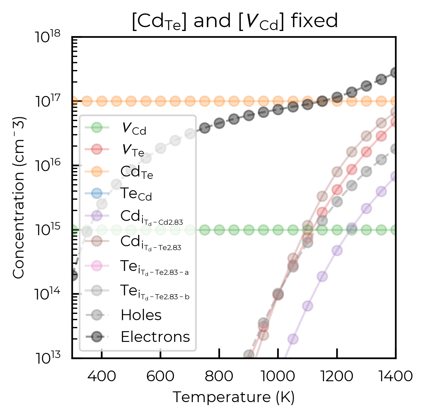
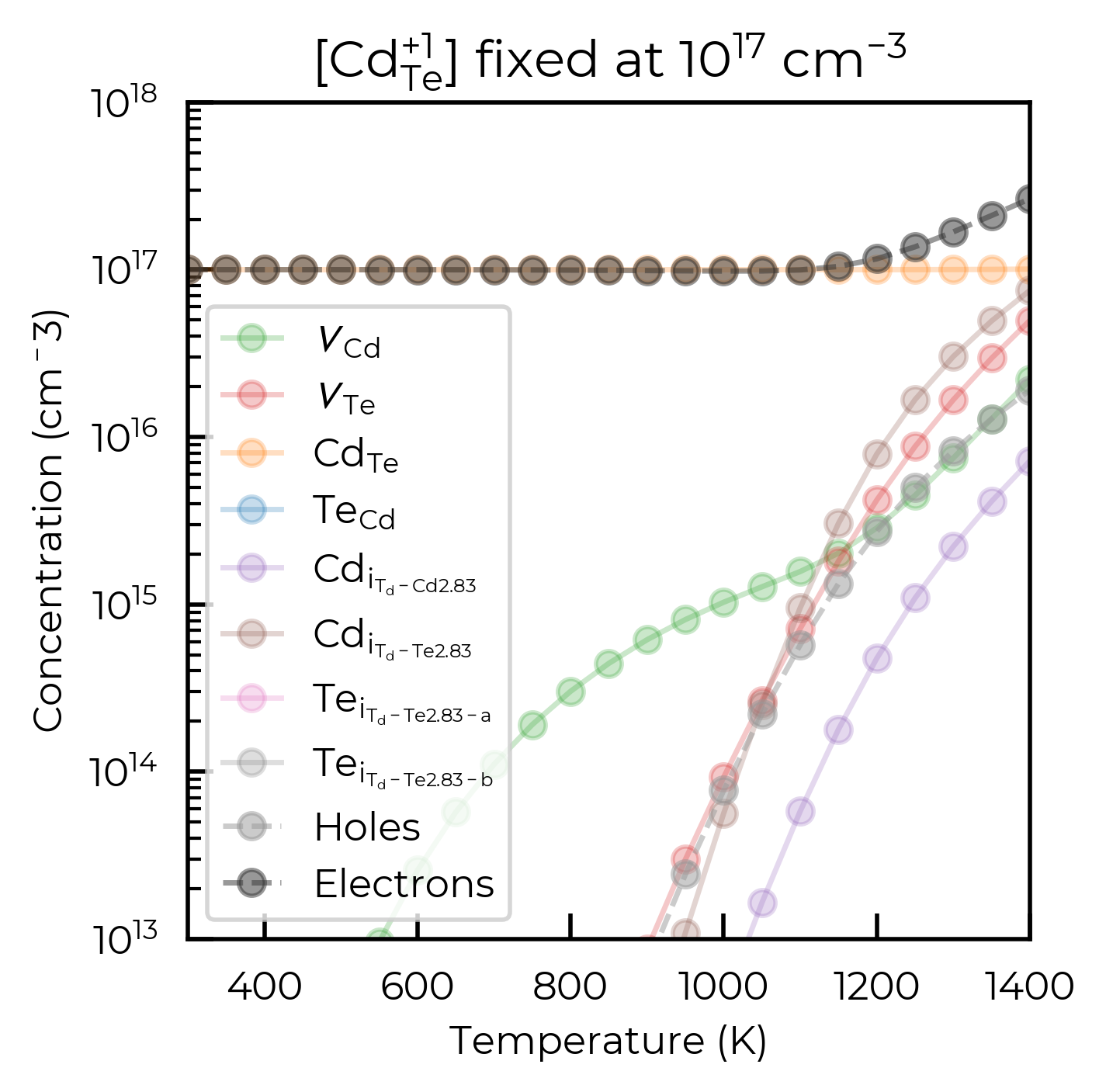
Another thing that can be customized in the ensembles is the addition of a fixed-defects argument. This also requires the use of the ps-sc-fermi back end. While the example we provide below are purely illustrative, these calculations can be used as a way to simulate the effect of a fixed-concentration impurity. This can either be done as a fixed concentration of a particular defect, or defect charge state, as illustrated in the cell below.
import numpy as np
import matplotlib.pyplot as plt
from doped.utils.plotting import format_defect_name

# Define a range of temperatures to scan over (in Kelvin)
temperatures = range(300, 1410, 50)

# First plot: Scan temperature with fixed defects {"Cd_Te": 1e17, "v_Cd": 1e15}
temperature_df_py = py_fs.scan_temperature(
    chempots={"Cd": 0.0, "Te": -1.2513},
    temperature_range=temperatures,
    fixed_defects={"Cd_Te": 1e17, "v_Cd": 1e15},
)

# Create unique list of defects and plot concentrations
fig, ax = plt.subplots()

# Plot the hole and electron concentrations
def plot_carrier_concentrations(plot_data, ax):
    ax.plot(
        plot_data["Temperature (K)"], plot_data["Holes (cm^-3)"],
        marker="o", linestyle="--", color="#999999", alpha=0.5, label="Holes"
    )
    ax.plot(
        plot_data["Temperature (K)"], plot_data["Electrons (cm^-3)"],
        marker="o", linestyle="--", color="#333333", alpha=0.5, label="Electrons"
    )

def plot_temperature_df(temperature_df, ax):
    unique_defects = temperature_df.index.unique()
    for defect in unique_defects:
        plot_data = temperature_df.loc[defect]
        ax.plot(
            plot_data["Temperature (K)"],
            plot_data["Concentration (cm^-3)"],
            label=format_defect_name(defect, include_site_info=True, wout_charge=True),
            color=defect_colors.get(defect, "C7"),
            marker="o",
            alpha=0.25,
        )
    plot_carrier_concentrations(plot_data, ax)

    # Set plot labels and scaling
    ax.set_xlabel("Temperature (K)"); ax.set_ylabel("Concentration (cm$^{-3}$)")
    ax.set_xlim(300, 1400); ax.set_ylim(1e13, 1e18)
    ax.set_yscale("log")
    ax.legend()

plot_temperature_df(temperature_df_py, ax)
plt.title(
    f"[{format_defect_name('Cd_Te', wout_charge=True)}] and [{format_defect_name('v_Cd', wout_charge=True)}] fixed"
)
plt.show()

# Second plot: Scan temperature with fixed defect {"Cd_Te_+1": 1e17}
temperature_df_py = py_fs.scan_temperature(
    chempots={"Cd": 0.0, "Te": -1.2513}, temperature_range=temperatures, fixed_defects={"Cd_Te_+1": 1e17}
)

fig, ax = plt.subplots()
plot_temperature_df(temperature_df_py, ax)
plt.title(rf"[{format_defect_name('Cd_Te_+1')}] fixed at $10^{{{17}}}$ cm$^{{{-3}}}$")
plt.show()
100%|██████████| 23/23 [00:01<00:00, 18.57it/s]
100%|██████████| 23/23 [00:01<00:00, 12.86it/s]
Cu2SiSe3: 2D Chemical Potential Scans
Another thing that has been added with the FermiSolver class is the ability to simply perform scans over >2d chemical potential spaces, this is outlined for Cu2SiSe3 (a potential solar absorber material) in the cells below.
The defect formation energy diagram for this system (left = Cu-poor; right = Cu-rich):

from monty.serialization import loadfn

# we need to specify the path to the vasprun.xml(.gz) file
# that was used for the DOS calculation. This is because
# we need to accurately account for the electronic carrier concentrations
# as well as the defect concentrations to determine the Fermi level
vasprun_path = "Cu2SiSe3/vasprun.xml.gz"

# the DefectThermodynamics object contains all the information about the
# defect formation energies and transition levels. It will underpin both the
# doped and py-sc-fermi solvers
defect_thermo = loadfn("Cu2SiSe3/Cu2SiSe3_thermo.json")

# In this case, our chempots have already been set as `DefectThermodynamics.chempots`,
# so we don't need to reload/set them, but if we wanted to, we could do so with:
# chempots = loadfn("Cu2SiSe3/Cu2SiSe3_chempots.json")
# defect_thermo.chempots = chempots

fs = FermiSolver(defect_thermodynamics=defect_thermo, bulk_dos=vasprun_path)
data = fs.scan_chemical_potential_grid(
    n_points=500,  # approx number of grid points to generate (can change due to duplicates etc)
    cartesian=True,  # default (barycentric, non-Cartesian) is usually best for efficiency, but Cartesian better for plotting here
    annealing_temperature=1000,  # the temperature at which to anneal the system
    quenched_temperature=300,  # the temperature at which to quench the system
)
100%|██████████| 497/497 [00:23<00:00, 21.25it/s]
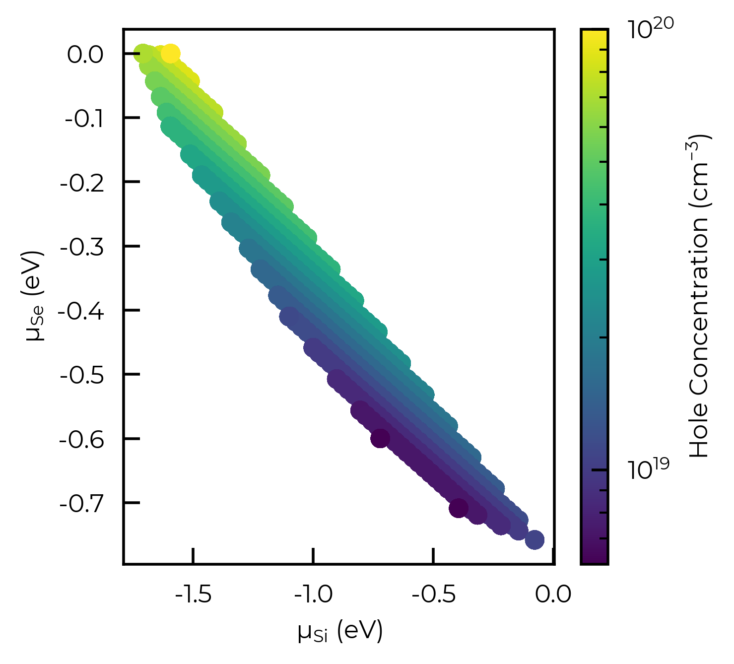
This can then be used to plot a variable of interest over the calculated points.
from matplotlib.colors import LogNorm

hole_concs = data["Holes (cm^-3)"]
plt.scatter(data["μ_Si (eV)"], data["μ_Se (eV)"], c=hole_concs, cmap='viridis',
            norm=LogNorm(min(hole_concs), 10**round(np.log10(max(hole_concs))))  # set upper limit to next order of magnitude for clearer colourbar here
)
cbar = plt.colorbar(label="Hole Concentration (cm$^{-3}$)")

plt.xlabel("μ$_{Si}$ (eV)"); plt.ylabel("μ$_{Se}$ (eV)")
plt.show()
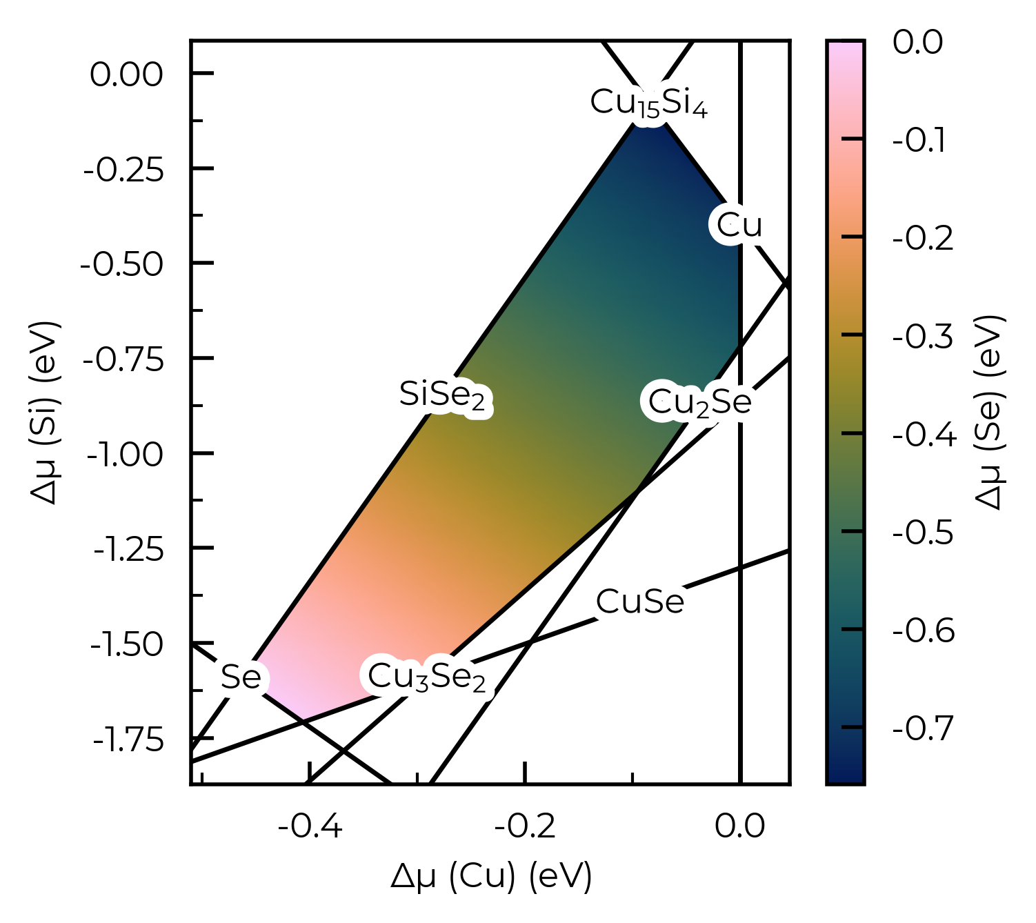
We can use the plot_chempot_heatmap method for DefectThermodynamics to compare this to the chemical potentials over the same region:
fs.defect_thermodynamics.plot_chempot_heatmap(dependent_element="Cu")
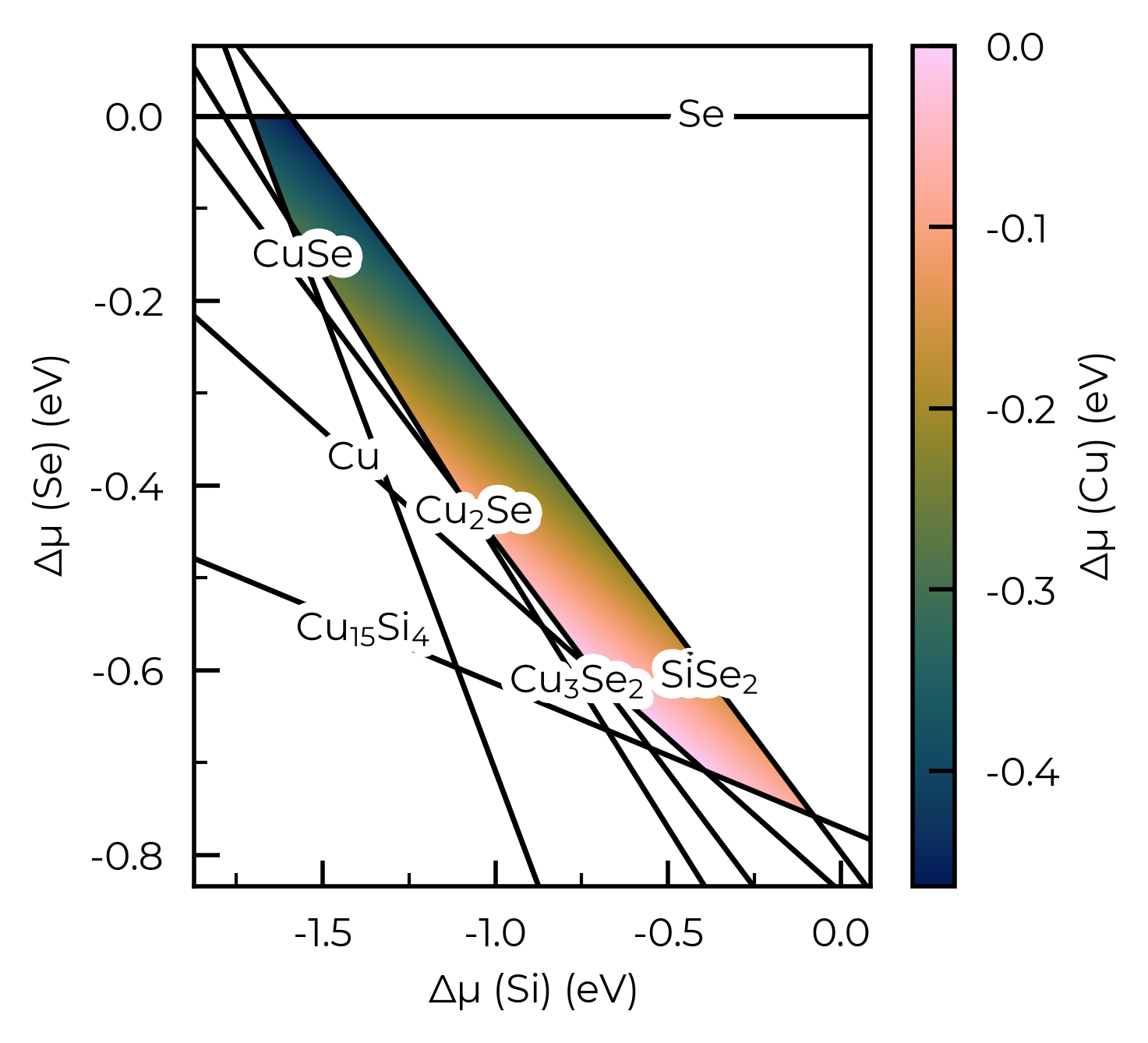
Here we see that the hole concentration follows the opposite trend to the Cu chemical potential, due to the fact that \(V\)Cu is the dominant acceptor species in this system (see formation energy diagram above), and so lower Cu chemical potentials (more Cu-poor conditions) favour higher copper vacancy and thus hole concentrations.
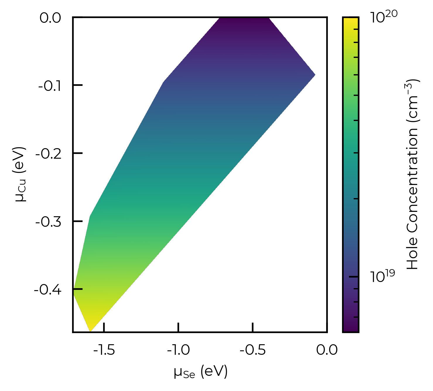
Same plot but using imshow to generate a smooth heatmap, and showing the Copper chemical potential on the y-axis (to illustrate the connection to the hole concentrations):
import numpy as np
from scipy.interpolate import griddata

f, ax = plt.subplots()
x = np.linspace(data["μ_Si (eV)"].min(), data["μ_Si (eV)"].max(), 1000)
y = np.linspace(data["μ_Cu (eV)"].min(), data["μ_Cu (eV)"].max(), 1000)
X, Y = np.meshgrid(x, y)

# Interpolate:
Z = griddata((data["μ_Si (eV)"], data["μ_Cu (eV)"]), data["Holes (cm^-3)"], (X, Y), method="cubic")
im = ax.imshow(
    Z,
    extent=(
        data["μ_Si (eV)"].min(),
        data["μ_Si (eV)"].max(),
        data["μ_Cu (eV)"].min(),
        data["μ_Cu (eV)"].max(),
    ),
    origin="lower",
    cmap="viridis",
    aspect="auto",
    norm=LogNorm(min(data["Holes (cm^-3)"]), 10 ** round(np.log10(max(data["Holes (cm^-3)"])))),
)
f.colorbar(im, label="Hole Concentration (cm$^{-3}$)")
ax.set_xlabel("μ$_{Se}$ (eV)"); ax.set_ylabel("μ$_{Cu}$ (eV)")
ax.set_xlim(ax.get_xlim()[0], 0)  # ensure x-axis extends to 0
plt.show()
Tip
Examples of plotting the chemical potentials as a heatmap for >=3D (i.e. >=ternary) systems are shown in the chemical potentials tutorial, while customisation of the heatmap plots is exemplified in the plotting customisation tutorial.
# one can also plot the chemical potential heatmap directly from the chempots dict:
from doped.chemical_potentials import plot_chempot_heatmap

chempots = loadfn("Cu2SiSe3/Cu2SiSe3_chempots.json")
chempot_plot = plot_chempot_heatmap(chempots, composition="Cu2SiSe3")
In these final cells, we show a tool for investigating complex chemical potential spaces. For a target value (hole, electron, or a specific defect concentration, or the Fermi energy) we find the position in chemical potential space where that target value is minimised or maximised. This is done by carrying out a coarse interpolation in chemical potential space, and finding an initial point at which the target value is minimised or maximised. A new chemical potential grid is then generated centered on this new value and the search repeated. This is done until the change in the target value is smaller than a provided tolerance factor. The output of the code is a dataframe that describes the defect system at the identified chemical potential. Example useage is shown in the cell below
max_holes_df = fs.optimise(
    target="Holes (cm^-3)",  # the target variable
    min_or_max="max",  # whether to find the minimum or maximum of the target variable
    tolerance=0.001,  # the convergence tolerance for the target variable, in relative magnitude
    annealing_temperature=1000,
    quenched_temperature=300,
)
max_holes_df
100%|██████████| 39/39 [00:01<00:00, 21.83it/s]
Searching for chemical potentials which maximise the target column: ['Holes (cm^-3)']...
100%|██████████| 39/39 [00:01<00:00, 24.16it/s]
| Concentration (cm^-3) | Annealing Temperature (K) | Quenched Temperature (K) | Fermi Level (eV wrt VBM) | Electrons (cm^-3) | Holes (cm^-3) | μ_Cu (eV) | μ_Si (eV) | μ_Se (eV) | |
|---|---|---|---|---|---|---|---|---|---|
| Defect | |||||||||
| v_Cu_1 | 9.918464e+19 | 1000 | 300 | -0.074357 | 2.704418e-10 | 9.905554e+19 | -0.463558 | -1.594069 | 0.0 |
| v_Si | 8.812211e+14 | 1000 | 300 | -0.074357 | 2.704418e-10 | 9.905554e+19 | -0.463558 | -1.594069 | 0.0 |
| v_Se | 4.554869e+11 | 1000 | 300 | -0.074357 | 2.704418e-10 | 9.905554e+19 | -0.463558 | -1.594069 | 0.0 |
| Cu_Si | 7.536802e+17 | 1000 | 300 | -0.074357 | 2.704418e-10 | 9.905554e+19 | -0.463558 | -1.594069 | 0.0 |
| Si_Cu | 2.095310e+06 | 1000 | 300 | -0.074357 | 2.704418e-10 | 9.905554e+19 | -0.463558 | -1.594069 | 0.0 |
| Si_Se | 1.828131e+02 | 1000 | 300 | -0.074357 | 2.704418e-10 | 9.905554e+19 | -0.463558 | -1.594069 | 0.0 |
| Se_Cu | 1.259815e+14 | 1000 | 300 | -0.074357 | 2.704418e-10 | 9.905554e+19 | -0.463558 | -1.594069 | 0.0 |
| Se_Si | 3.275868e+16 | 1000 | 300 | -0.074357 | 2.704418e-10 | 9.905554e+19 | -0.463558 | -1.594069 | 0.0 |
| Int_Cu | 1.287555e+17 | 1000 | 300 | -0.074357 | 2.704418e-10 | 9.905554e+19 | -0.463558 | -1.594069 | 0.0 |
| Int_Si | 1.931946e+02 | 1000 | 300 | -0.074357 | 2.704418e-10 | 9.905554e+19 | -0.463558 | -1.594069 | 0.0 |
| Int_Se | 5.145858e+13 | 1000 | 300 | -0.074357 | 2.704418e-10 | 9.905554e+19 | -0.463558 | -1.594069 | 0.0 |
As expected, we see our target variable (the hole concentration here) is maximised for low copper chemical potentials (μCu = -0.46 eV) which corresponds to copper-poor conditions.
Tip
The delta_VBM/delta_CBM arguments used in DefectThermodynamics.get_fermi_level_and_concentrations() are also supported by all FermiSolver scan methods (scan_temperature, scan_chempots, interpolate_chempots, etc.), and can be either floats or callables of (annealing) temperature – see the ZGO example below and the thermodynamics tutorial for further discussion.
Extremal concentrations at non-limiting chemical potentials: \(V_S\) in Sb₂S₃
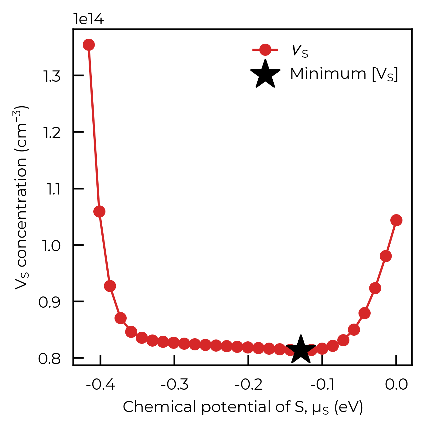
In the example above, the target variable (the hole concentration) was extremised at one of the chemical-potential limits (Cu-poor conditions). This is not always the case, and in many cases a carrier/defect concentration can be maximised/minimised at an internal / non-limiting chemical potential! (i.e. a chemical potential within the chemical stability region, rather than at the edge/vertex).
One example is the sulfur vacancy (\(V_S\)) in Sb₂S₃, whose concentration is actually minimised at an intermediate chemical potential, rather than at either the S-rich or S-poor (Sb-rich) limit – see Figure 1 in ACS Energy Letters (2024). Similar behaviour is discussed for \(V_{Se}\) in the sister compound Sb₂Se₃, where more selenium vacancies were predicted to form under Se-rich conditions – see Small (2021).
The optimise function can natively locate such non-trivial extrema in chemical-potential space, where a simple comparison of the limiting conditions would give an incomplete story:
from monty.serialization import loadfn
from doped.thermodynamics import FermiSolver
# the Sb2S3 DefectThermodynamics already has its chempots and bulk DOS embedded:
sb2s3_thermo = loadfn("Sb2S3/Sb2S3_thermo.json.gz")
sb2s3_fs = FermiSolver(sb2s3_thermo)

# find the chemical potentials that minimise the V_S_3 concentration (the dominant
# sulfur vacancy), under annealing at 603 K and quenching to 300 K:
min_V_S_df = sb2s3_fs.optimise(
    target="V_S_3",  # the target defect (without charge state)
    min_or_max="min",  # minimise its concentration
    annealing_temperature=603,
    quenched_temperature=300,
    per_charge=False,
)
min_V_S_df
100%|██████████| 30/30 [00:02<00:00, 13.51it/s]
Searching for chemical potentials which minimise the target defect(s): ['V_S_3']...
100%|██████████| 30/30 [00:02<00:00, 12.77it/s]
| Concentration (cm^-3) | Annealing Temperature (K) | Quenched Temperature (K) | Fermi Level (eV wrt VBM) | Electrons (cm^-3) | Holes (cm^-3) | μ_Sb (eV) | μ_S (eV) | |
|---|---|---|---|---|---|---|---|---|
| Defect | ||||||||
| V_S_1 | 1.637373e+12 | 603 | 300 | 0.75778 | 63.268708 | 821421.380627 | -0.430446 | -0.129134 |
| V_S_2 | 4.990283e+13 | 603 | 300 | 0.75778 | 63.268708 | 821421.380627 | -0.430446 | -0.129134 |
| V_S_3 | 8.141019e+13 | 603 | 300 | 0.75778 | 63.268708 | 821421.380627 | -0.430446 | -0.129134 |
| V_Sb_1 | 8.763541e+13 | 603 | 300 | 0.75778 | 63.268708 | 821421.380627 | -0.430446 | -0.129134 |
| V_Sb_2 | 1.046441e+13 | 603 | 300 | 0.75778 | 63.268708 | 821421.380627 | -0.430446 | -0.129134 |
| S_Sb_1 | 9.096801e+12 | 603 | 300 | 0.75778 | 63.268708 | 821421.380627 | -0.430446 | -0.129134 |
| S_Sb_2 | 7.195315e+10 | 603 | 300 | 0.75778 | 63.268708 | 821421.380627 | -0.430446 | -0.129134 |
| Sb_S_1 | 6.540701e+05 | 603 | 300 | 0.75778 | 63.268708 | 821421.380627 | -0.430446 | -0.129134 |
| Sb_S_2 | 1.634560e+09 | 603 | 300 | 0.75778 | 63.268708 | 821421.380627 | -0.430446 | -0.129134 |
| Sb_S_3 | 2.399022e+07 | 603 | 300 | 0.75778 | 63.268708 | 821421.380627 | -0.430446 | -0.129134 |
| Int_S_5 | 2.960823e-09 | 603 | 300 | 0.75778 | 63.268708 | 821421.380627 | -0.430446 | -0.129134 |
| Int_S_9 | 8.489646e+11 | 603 | 300 | 0.75778 | 63.268708 | 821421.380627 | -0.430446 | -0.129134 |
| Int_Sb_1 | 2.620774e+09 | 603 | 300 | 0.75778 | 63.268708 | 821421.380627 | -0.430446 | -0.129134 |
The output dataframe describes the full defect system at the identified chemical potentials. Pulling out the target defect, we can see that \(V_S\) is minimised at an intermediate chemical potential (\(\mu_{Sb} \approx -0.43\) eV, \(\mu_S \approx -0.13\) eV), well away from either limit:
opt_row = min_V_S_df.loc["V_S_3"]
opt_mu_S = opt_row["μ_S (eV)"]
opt_conc = opt_row["Concentration (cm^-3)"]
print(
    f"V_S_3 minimised at μ_Sb = {opt_row['μ_Sb (eV)']:.3f} eV, "
    f"μ_S = {opt_mu_S:.3f} eV  (concentration = {opt_conc:.2e} cm⁻³)"
)
V_S_3 minimised at μ_Sb = -0.430 eV, μ_S = -0.129 eV (concentration = 8.14e+13 cm⁻³)
To verify that this is indeed the true minimum, we can scan over the full chemical-potential range between the Sb-rich and S-rich limits using interpolate_chempots, plot the \(V_S\) concentration as a function of \(\mu_S\), and mark the optimise result. As expected, the optimise point sits right at the bottom of the U-shaped curve, at an intermediate \(\mu_S\):
import matplotlib.pyplot as plt
from doped.utils.plotting import format_defect_name
# scan the full chempot range between the Sb-rich and S-rich limits:
scan_df = sb2s3_fs.interpolate_chempots(
    limits=["Sb2S3-Sb", "Sb2S3-S"], n_points=30,
    annealing_temperature=603, quenched_temperature=300, per_charge=False,
)
V_S_3_scan = scan_df.loc["V_S_3"]

fig, ax = plt.subplots()
ax.plot(
    V_S_3_scan["μ_S (eV)"],
    V_S_3_scan["Concentration (cm^-3)"],
    marker="o",
    color="C3",
    label=format_defect_name("V_S_3", wout_charge=True),
)

# mark the chemical potential identified by ``optimise``:
ax.scatter(opt_mu_S, opt_conc, marker="*", s=300, color="k", zorder=5, label="Minimum [V$_S$]")

ax.set_xlabel("Chemical potential of S, $\\mu_S$ (eV)")
ax.set_ylabel("$V_S$ concentration (cm$^{-3}$)")
ax.legend(frameon=False)
plt.show()
100%|██████████| 30/30 [00:02<00:00, 13.36it/s]
Notably, the occurrence of defect/carrier concentration extrema at non-limiting chemical potentials is far more likely with multinary compositions, due to greater complexity with more chemical potential dimensions, and so it is highly recommended to use the scan_chemical_potential_grid and optimise FermiSolver methods in these cases to fully navigate and probe the accessible defect/carrier concentrations for your system.
Complex Quinary: Na2FePO4F
These classes and functions can equally be used with more complex multinary systems. Here we take the quinary Na2FePO4F as an example. Let’s generate a ChemicalPotentialGrid for this system using data from the Materials Project (note that typically, of course, we would use the CompetingPhases class to generate input files for the relevant secondary/competing phases and calculate these with our chosen settings, before parsing with CompetingPhasesAnalyzer, but here we use MP data for a quick example):
from doped import chemical_potentials

na2fepo4f_cp = chemical_potentials.CompetingPhases("Na2FePO4F")  # get
na2fepo4f_doped_chempots = chemical_potentials.get_doped_chempots_from_entries(
    na2fepo4f_cp.entries, "Na2FePO4F"
)
na2fepo4f_grid = chemical_potentials.ChemicalPotentialGrid(na2fepo4f_doped_chempots)

# alternatively we could initialise the grid with:
na2fepo4f_cpa = chemical_potentials.CompetingPhasesAnalyzer("Na2FePO4F", entries=na2fepo4f_cp.entries)
na2fepo4f_grid = na2fepo4f_cpa.chempot_grid
The ChemicalPotentialGrid object is used internally in many of the FermiSolver methods, but can also be useful for manual / advanced analyses of chemical potentials and the behaviour of various properties as a function of chemical potentials.
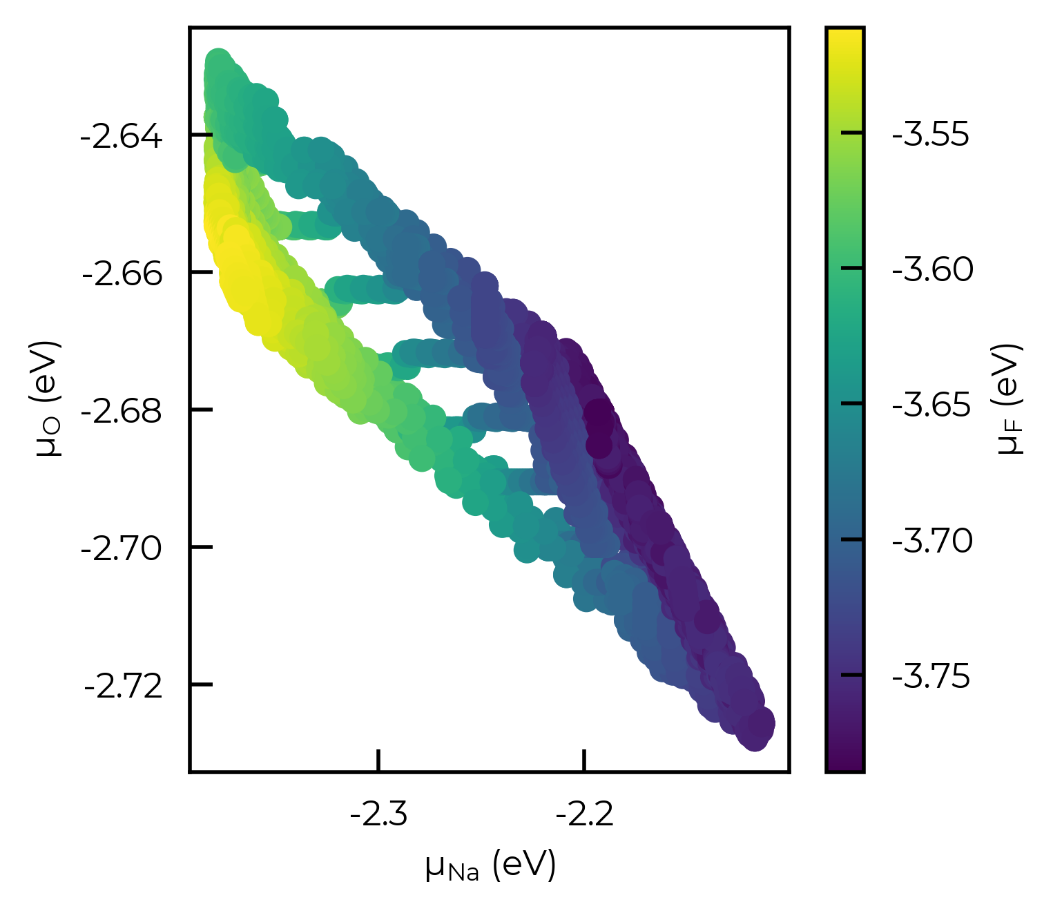
Here as an example we will manually plot the Fluorine chemical potential as a function of the Na and O chemical potentials, with Fe and P chemical potentials fixed at their mid-range values:
grid_df = na2fepo4f_grid.get_grid(1e8, drop_duplicates=False) # generate dense grid
import matplotlib.pyplot as plt
import numpy as np

middle_mu_Fe = grid_df["μ_Fe (eV)"].min() + (grid_df["μ_Fe (eV)"].max() - grid_df["μ_Fe (eV)"].min()) / 2
middle_mu_P = grid_df["μ_P (eV)"].min() + (grid_df["μ_P (eV)"].max() - grid_df["μ_P (eV)"].min()) / 2

fixed_chempot_df = grid_df[
    (np.isclose(grid_df["μ_Fe (eV)"], middle_mu_Fe, atol=0.01))
    & (np.isclose(grid_df["μ_P (eV)"], middle_mu_P, atol=0.01))
]

fig, ax = plt.subplots()
sc = ax.scatter(
    fixed_chempot_df["μ_Na (eV)"],
    fixed_chempot_df["μ_O (eV)"],
    c=fixed_chempot_df["μ_F (eV)"],
    cmap="viridis",
)
fig.colorbar(sc, ax=ax, label="μ$_F$ (eV)")
ax.set_xlabel("μ$_{Na}$ (eV)")
ax.set_ylabel("μ$_{O}$ (eV)");
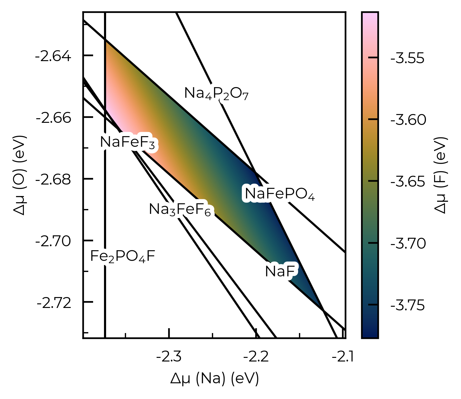
We could also use the plot_chempot_heatmap method for CompetingPhasesAnalyzer to do this too:
chempot_heatmap = na2fepo4f_cpa.plot_chempot_heatmap(fixed_elements={"Fe": middle_mu_Fe, "P": middle_mu_P})
ZGO: Asymmetric Band-Edge Renormalisation with scan_temperature
The thermodynamics tutorial demonstrates accounting for asymmetric, temperature-dependent band-edge renormalisation in ZnGa₂O₄ (ZGO; Claes et al. ACS Appl. Mater. Interfaces 2025) via direct calls to DefectThermodynamics.get_fermi_level_and_concentrations – see that section for more discussion. The same physics is fully supported by FermiSolver.scan_temperature (and all other FermiSolver scan/optimise methods) – with delta_VBM/delta_CBM accepted as constants or as functions of annealing temperature, so a single call efficiently performs the full sweep:
import numpy as np
from monty.serialization import loadfn

from doped.thermodynamics import FermiSolver

ZGO_thermo = loadfn("ZGO/ZGO_thermo.json.gz")
ZGO_thermo.bulk_dos = "ZGO/ZGO_bulk_DOS_vasprun.xml.gz"
ZGO_solver = FermiSolver(ZGO_thermo)

# Linear fits to e-ph-derived VBM(T) and CBM(T) shifts in ZGO (eV, T in K);
# the VBM shifts up while the CBM shifts down (gap shrinks asymmetrically with T)
def VBM_shift(T):
    return 0.196 + 2.85e-4 * T

def CBM_shift(T):
    return -0.0935 - 1.97e-4 * T

def delta_gap(T):  # equivalent symmetric gap change, for comparison
    return CBM_shift(T) - VBM_shift(T)
Compared with calling get_fermi_level_and_concentrations in a Python loop (as in the thermodynamics tutorial), FermiSolver.scan_temperature performs the full sweep in one call, with the same delta_VBM/delta_CBM callable accepted as a function of annealing temperature. The same applies to the other FermiSolver scanning/optimisation methods (scan_chempots, interpolate_chempots, scan_chemical_potential_grid, optimise, etc.).
anneal_temperatures = np.arange(300, 2101, 50)
common_kwargs = {
    "annealing_temperature_range": anneal_temperatures,
    "chempots": ZGO_thermo.chempots,
    "limit": "Zn(GaO2)2-Zn-Ga",
    "per_charge": False,
    "return_annealing_values": True,
}
# No renormalisation, symmetric, and full asymmetric renormalisation of the band edges:
df_none = ZGO_solver.scan_temperature(**common_kwargs)
df_sym = ZGO_solver.scan_temperature(
    **common_kwargs,
    delta_VBM=lambda T: -delta_gap(T) / 2,
    delta_CBM=lambda T: delta_gap(T) / 2,
)
df_asym = ZGO_solver.scan_temperature(
    **common_kwargs,
    delta_VBM=VBM_shift,
    delta_CBM=CBM_shift,
)
  0%|          | 0/37 [00:00<?, ?it/s]The defect supercell has been detected to possibly have a non-scalar matrix expansion, which could be breaking the cell periodicity and possibly preventing the correct _relaxed_ point group symmetries (and thus orientational degeneracies) from being automatically determined.
This will not affect defect formation energies / transition levels, but can be important for concentrations/doping/Fermi level behaviour (10.1039/D2FD00043A, 10.1039/D3CS00432E, 10.1038/s41578-025-00879-y ...).
You can manually check (and edit) the computed defect point symmetries and corresponding orientational degeneracy factors by inspecting/editing the calculation_metadata['relaxed point symmetry'] and degeneracy_factors['orientational degeneracy'] attributes.
100%|██████████| 37/37 [00:01<00:00, 27.32it/s]
100%|██████████| 37/37 [00:01<00:00, 26.47it/s]
100%|██████████| 37/37 [00:01<00:00, 28.93it/s]
Defect & carrier concentrations: no/symmetric/full (asymmetric) renormalisation
The figure below reproduces Fig. S6 of Claes et al., comparing the temperature dependence of the dominant intrinsic defect populations and electron concentration for the three band-edge renormalisation cases:
import matplotlib.pyplot as plt
import doped
from doped.utils.plotting import shade_band_edges

plt.style.use(f"{doped.__path__[0]}/utils/doped.mplstyle")  # use doped style

n_exp_low, n_exp_high = 5e18, 5e19  # cm^-3 (Claes et al. Fig. 1)

def n_quench_vs_T(df):
    return df.groupby("Annealing Temperature (K)")["Electrons (cm^-3)"].first().to_numpy()

def conc_vs_T(df, defect_name):
    """Annealing-frozen total concentration vs T for a given defect."""
    if defect_name not in df.index.get_level_values("Defect"):
        return np.full(len(anneal_temperatures), np.nan)
    sub = df.loc[defect_name]
    return (
        sub.set_index("Annealing Temperature (K)")
        .loc[anneal_temperatures, "Concentration (cm^-3)"]
        .to_numpy()
    )

defect_styles = {
    "Ga_Zn": ("tab:purple", r"Ga$_{\mathrm{Zn}}$"),
    "Zn_Ga": ("tab:red", r"Zn$_{\mathrm{Ga}}$"),
    "v_Zn": ("tab:blue", r"v$_{\mathrm{Zn}}$"),
    "v_O": ("tab:green", r"v$_{\mathrm{O}}$"),
    "v_Ga": ("tab:orange", r"v$_{\mathrm{Ga}}$"),
}

panels = [
    (df_none, "No renormalization"),
    (df_sym, "Symmetric renormalization"),
    (df_asym, "Asymmetric renormalization"),
]

f, axes = plt.subplots(1, 3, figsize=(11, 3), sharey=True, constrained_layout=True)
for ax, (df, title) in zip(axes, panels):
    ax.axhspan(n_exp_low, n_exp_high, color="teal", alpha=0.25, label="Expt. $n$")
    n_quench = n_quench_vs_T(df)
    n_anneal = df.groupby("Annealing Temperature (K)")["Electrons @ T_Anneal"].first().to_numpy()
    ax.semilogy(anneal_temperatures, n_quench, ls="--", lw=2, color="teal", label="n")
    ax.semilogy(
        anneal_temperatures,
        n_anneal,
        ls="--",
        lw=1.2,
        color="teal",
        alpha=0.5,
        label=r"n (T$_{\mathrm{anneal}}$)",
    )
    for d_name, (color, label) in defect_styles.items():
        ax.semilogy(
            anneal_temperatures,
            conc_vs_T(df, d_name),
            marker="o",
            markersize=4,
            ls="--",
            lw=0.8,
            color=color,
            label=label,
        )
    ax.set_title(title)
    ax.set_xlabel("Processing Temperature (K)")
    ax.set_xlim(300, 2100)
axes[0].set_ylabel("Concentration (cm$^{-3}$)")
axes[0].set_ylim(1e14, 1e22)
# Single shared legend using handles from the middle panel:
handles, labels = axes[1].get_legend_handles_labels()
axes[-1].legend(handles, labels, bbox_to_anchor=(1.02, 1), loc="upper left", frameon=False)
plt.show()
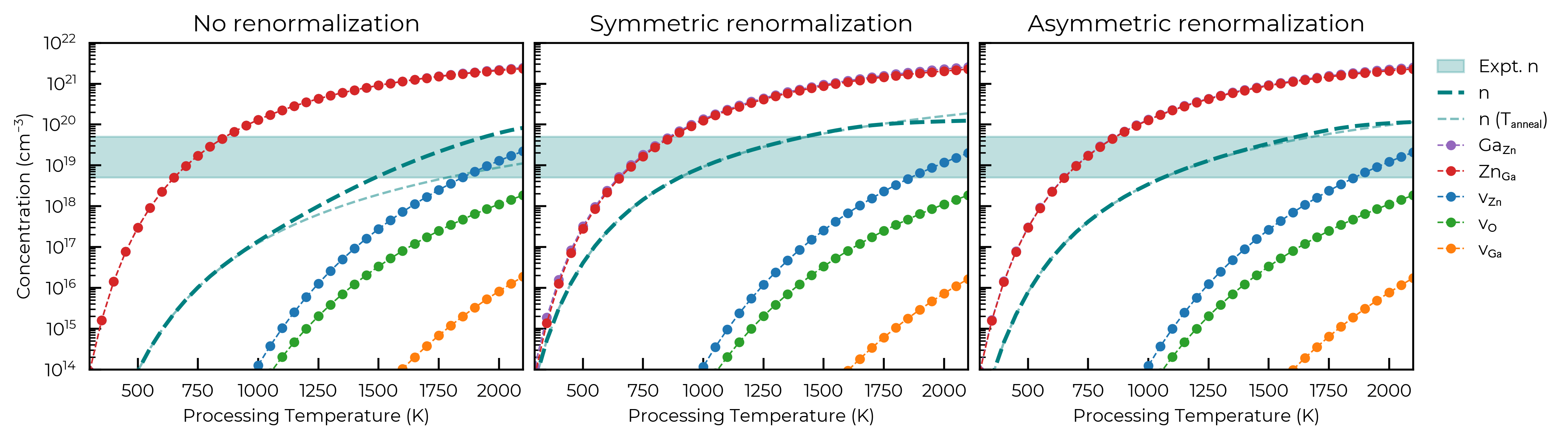
Note
Here for illustration we compute three example scenarios; with no band-edge temperature effects, with symmetric band-edge renormalisation and with full asymmetric band-edge renormalisation. In an actual research investigation of course, you would likely just use the highest fidelity data you have available!