Competing Phases
To calculate the limiting chemical potentials of elements in the material (needed for calculating the defect formation energies) we need to consider the energies of all competing phases. doped does this by calling the CompetingPhases class, which then queries Materials Project to obtain all the relevant competing phases to be calculated.
In some cases the Materials Project may not have all known phases in a certain chemical space, so it’s a good idea to cross-check the generated competing phases with the ICSD in case you suspect any are missing.
For this functionality to work correctly, you will need an API key for the Materials Project (as described on the Installation docs page).
Tip
You can run this notebook interactively through Google Colab or Binder – just click the links! (Then uncomment the !pip install... cell).
# # If running on Colab; uncomment to install doped, clone the repo to download the example data and cd in to examples folder:
# !pip install doped
# !git clone https://github.com/SMTG-Bham/doped
# %cd doped/examples
# # Note that when running on Colab, POTCAR file generation will not be possible as this requires the VASP POTCAR directory
# # to be setup with pymatgen (see https://doped.readthedocs.io/en/latest/Installation.html), but all other parts of this
# # notebook can be run directly
from doped.chemical_potentials import CompetingPhases
For example, if we want to calculate the chemical potentials with ZrO2 as our host material, we would generate the relevant competing phases like so:
cp = CompetingPhases("ZrO2")  # default energy_above_hull = 0.05 eV/atom
# if you don't have your MP API key set up in ~/.pmgrc.yaml (see Installation docs),
# you can supply it as a parameter in this function, or set it as an env var with:
# !export MP_API_KEY="your_api_key"
Note
Note: The current algorithm for how doped queries the Materials Project (MP) and determines relevant competing phases to be calculated, is that it first queries the MP for all phases with energies above hull less than energy_above_hull eV/atom (optional parameter in CompetingPhases(); default is 0.05 eV/atom) in the chemical space of the host material.
It then determines which of these phases border the host material in the phase diagram (i.e. which are competing phases and thus determine the chemical potentials), as well as which phases would border the host material if their energies were downshifted by energy_above_hull. The latter are included as well, and so energy_above_hull acts as an uncertainty range for the MP-calculated formation energies, which may not be accurate due to functional choice (e.g. GGA vs hybrid DFT / GGA+U / RPA etc.), lack of vdW corrections etc.
The default energy_above_hull of 50 meV/atom works well in accounting for MP formation energy inaccuracies in most known cases. However, some critical thinking is key (as always!) and so if there are any obvious missing phases or known failures of the Materials Project energetics in your chemical space of interest, you should adjust this parameter to account for this (or alternatively manually include these known missing phases in your competing phase calculations, to be included in parsing and chemical potential analysis later on).
Particular attention should be paid for materials containing transition metals, (inter)metallic systems, mixed oxidation states, van der Waals (vdW) binding and/or large spin-orbit coupling (SOC) effects, for which the Materials Project energetics are typically less reliable.
Tip
In some cases, there are many metastable allotropes/polymorphs on the Materials Project database, which can result in a large number of competing phases to calculate and consider. The Chemical Systems with Many Polymorphs section at the bottom of this tutorial discusses some strategies for dealing with such cases.
Often energy_above_hull can be lowered (e.g. to 0) to reduce the number of calculations while retaining good accuracy relative to the typical error of defect calculations.
cp.entries contains pymatgen ComputedStructureEntry objects for all the relevant competing phases, which includes useful data such as their structures, magnetic moment and (MP-calculated GGA) band gaps.
print(len(cp.entries))
print([entry.name for entry in cp.entries])
18
['ZrO2', 'Zr', 'O2', 'Zr3O', 'Zr4O', 'Zr3O', 'Zr3O', 'Zr2O', 'ZrO2', 'ZrO2', 'Zr', 'ZrO2', 'ZrO2', 'ZrO2', 'ZrO2', 'ZrO2', 'Zr', 'ZrO2']
We can plot our phase diagram like this, which can show why certain phases are included as competing phases:
import doped
import matplotlib.pyplot as plt

plt.rcdefaults()
plt.style.use(f"{doped.__path__[0]}/utils/doped.mplstyle")  # use doped style
from mp_api.client import MPRester
from pymatgen.analysis.phase_diagram import PhaseDiagram, PDPlotter

system = ["Zr", "O"]  # system we want to get phase diagram for
mpr = MPRester()  # object for connecting to MP Rest interface, may need to specify API key here
entries = mpr.get_entries_in_chemsys(system)  # get all entries in the chemical system
pd = PhaseDiagram(entries)  # create phase diagram object
plotter = PDPlotter(pd, show_unstable=0.1, backend="matplotlib")  # plot phase diagram
plot = plotter.get_plot()
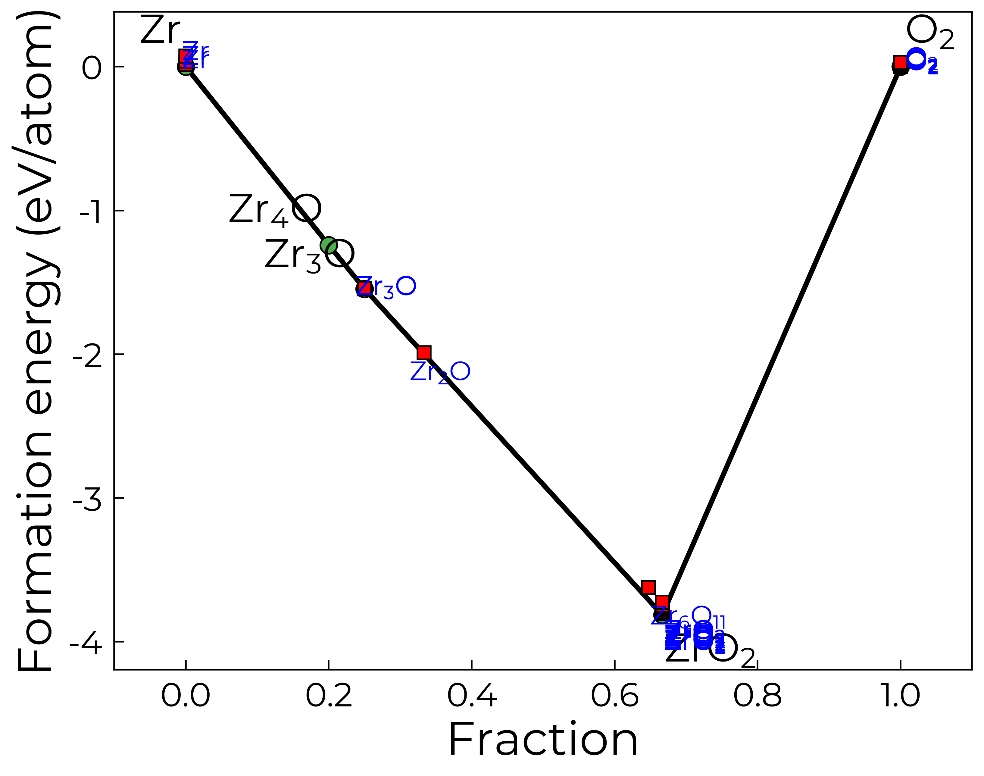
In this case, we see that there are many low-energy polymorphs of ZrO2 on the MP database. If for example we had already calculated the different polymorphs of ZrO2 and knew the MP-predicted groundstate (i.e. with MP-calculated energy above hull of zero) was indeed the groundstate with our chosen QM/DFT setup, we could then remove the extra ZrO2 phases here like so:
cp.entries = [entry for entry in cp.entries if entry.name != "ZrO2" or entry.data["energy_above_hull"] == 0]
print(len(cp.entries))
print([entry.name for entry in cp.entries])
10
['ZrO2', 'Zr', 'O2', 'Zr3O', 'Zr4O', 'Zr3O', 'Zr3O', 'Zr2O', 'Zr', 'Zr']
Similarly, if we had prior knowledge that the Materials Project data was accurate for our chosen host material, or were doing a high-throughput investigation where we were happy to sacrifice some accuracy/completeness for efficiency, we could set energy_above_hull to zero (i.e. total confidence in the MP data):
cp = CompetingPhases("ZrO2", energy_above_hull=0)
print(len(cp.entries))
print([entry.name for entry in cp.entries])
4
['ZrO2', 'Zr', 'O2', 'Zr3O']
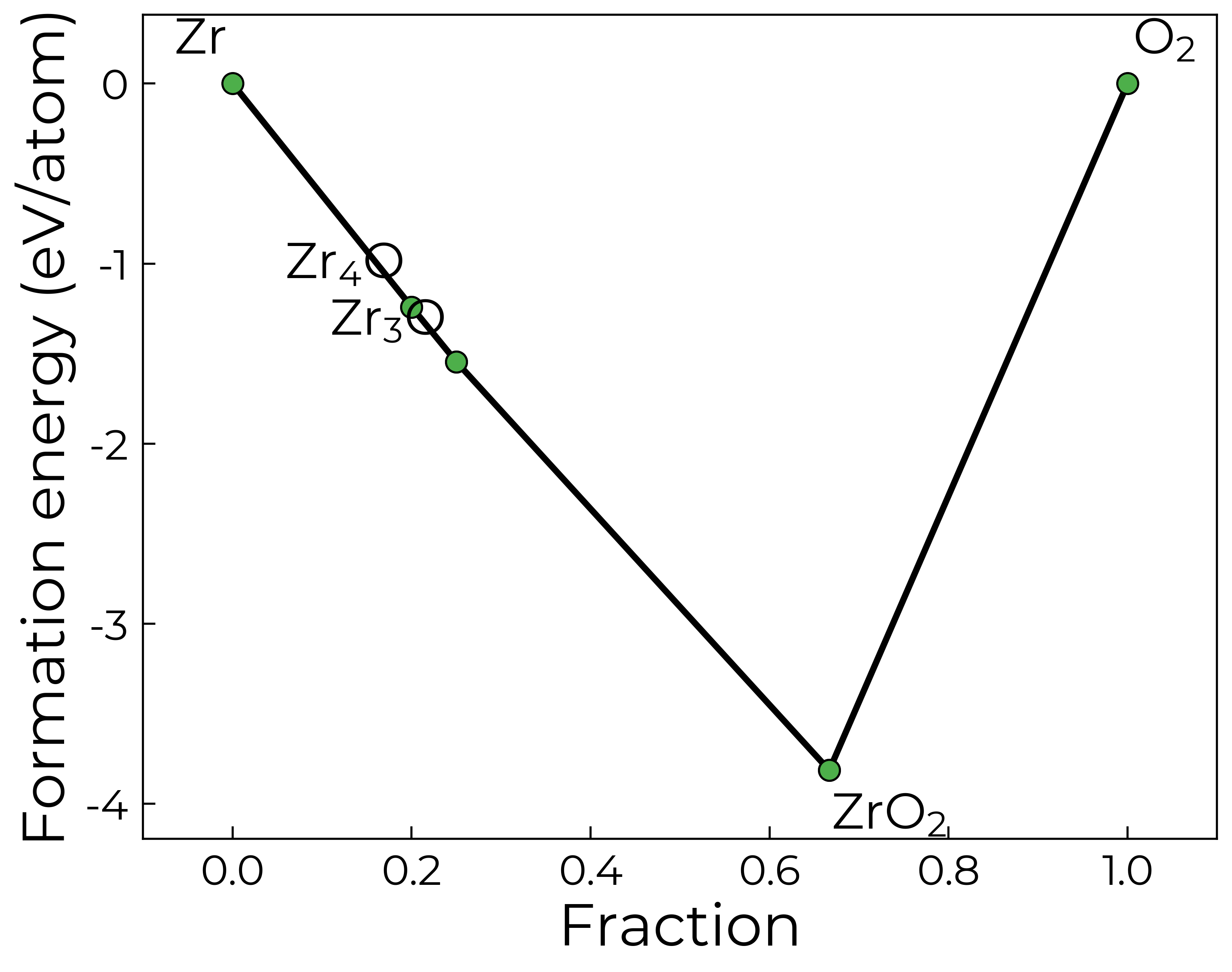
Indeed, if we plot our phase diagram again, only showing the stable MP entries, we see that only Zr3O and O2 border ZrO2, and so these (plus any remaining elements; i.e. Zr here) are the only competing phases generated with energy_above_hull = 0:
plotter = PDPlotter(pd, show_unstable=0, backend="matplotlib")  # plot phase diagram
plot = plotter.get_plot()
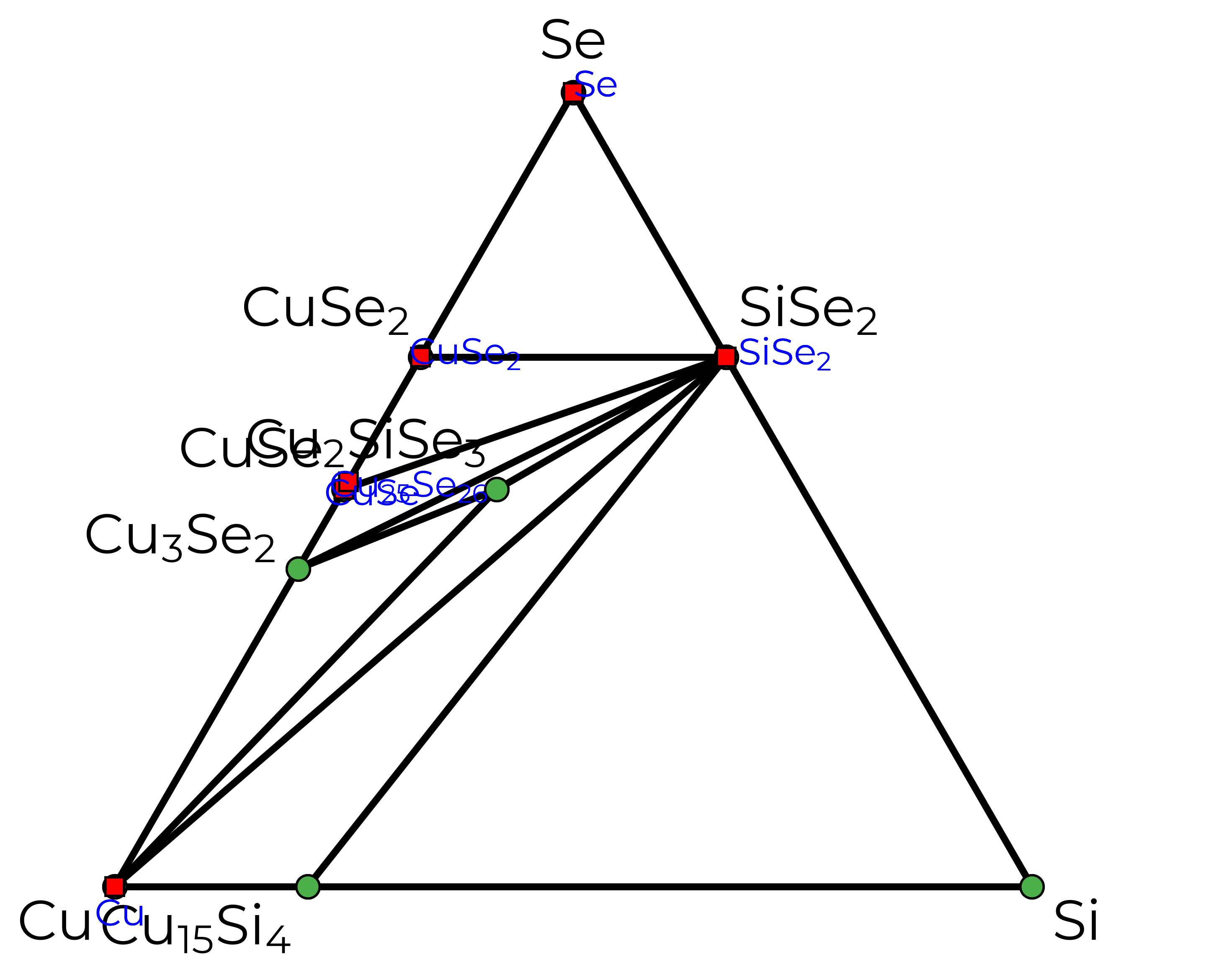
Just to illustrate, this is what our phase diagram would look like for a ternary system like Cu\(_2\)SiSe\(_3\) (a promising solar absorber):
system = ["Cu", "Si", "Se"]  # system we want to get phase diagram for
mpr = MPRester()  # object for connecting to MP Rest interface, may need to specify API key here
entries = mpr.get_entries_in_chemsys(system)  # get all entries in the chemical system
pd = PhaseDiagram(entries)  # create phase diagram object
plotter = PDPlotter(pd, show_unstable=0.01, backend="matplotlib")  # plot phase diagram
plot = plotter.get_plot()
Ignoring fixed y limits to fulfill fixed data aspect with adjustable data limits.
Generating input files
We can then set up the competing phase calculations with doped as described below, or use the pymatgen ComputedStructureEntry objects in cp.entries to set these up in your desired format with python / atomate / AiiDA etc.
k-points convergence testing is done at GGA (PBEsol by default) and is set up to account for magnetic moment convergence as well. Here we interface with vaspup2.0 to make it easy to use on the HPCs (with the generate-converge command to run the calculations and data-converge to quickly parse and analyse the results).
You may want to change the default ENCUT (350 eV) or k-point densities that the convergence tests span (5 - 120 kpoints/Å3 for semiconductors & insulators and 40 - 1000 kpoints/Å3 for metals). Note that ISMEAR is set to 0 (gaussian smearing) for semiconductors & insulators and 2 (2nd order Methfessel-Paxton smearing) for metals by default, following the recommended choices in VASP, and k-point convergence testing is not required for molecules (Γ-point sampling is sufficient).
Note that doped generates “molecule in a box” structures for the gaseous elemental phases
H2, O2, N2, F2 and Cl2. The molecule is placed in
a slightly-symmetry-broken (to avoid metastable electronic solutions) 30 Å cuboid box, and relaxed with Γ-point-only k-point sampling.
The kpoints convergence calculations are set up with:
Important
If the ground-state structure for your host composition is not listed on the Materials Project database (e.g. if you have a lower-symmetry lower-energy phase (common for perovskites for instance) or if it is a newly-discovered compound etc.), then you should use this structure for the competing phase energy calculation of your host composition (and, in most cases, for generating defect supercells), rather than the auto-generated Materials Project structure.
cp.convergence_setup(
    user_incar_settings={"GGA": "PE"},
    # potcar_spec=True  # uncomment to run on Colab!
)  # For custom INCAR settings, any flags that aren't numbers or True/False need to be input as strings with quotation marks
`CompetingPhases.convergence_setup` is deprecated and will be removed in the next minor release (v4.1); use `CompetingPhases.write_kpoint_convergence_files` instead.
Note that diatomic molecular phases, calculated as molecules-in-a-box (O2 in this case), do not require k-point convergence testing, as Γ-only sampling is sufficient.
{'CompetingPhases/ZrO2_P2_1c_EaH_0/kpoint_converge/k2,2,1': doped DopedDictSet with structure composition Zr4 O8. Available attributes:
 {'poscar_comment', 'charge_state', 'potcar_functional', 'user_potcar_settings', 'files_to_transfer', 'incar', 'poscar', 'kpoints_updates', 'incar_updates', 'prev_vasprun', 'config_dict', 'inherit_incar', 'bandgap', 'constrain_total_magmom', 'prev_incar', 'user_kpoints_settings', 'user_potcar_functional', 'vdw', 'auto_lreal', 'reduce_structure', 'auto_metal_kpoints', 'prev_outcar', 'structure', 'sym_prec', 'bandgap_tol', 'force_gamma', 'use_structure_charge', 'prev_kpoints', 'auto_kpar', 'auto_kspacing', 'kpoints', 'validate_magmom', 'auto_ismear', 'standardize', 'international_monoclinic', 'auto_ispin', 'sort_structure', 'nelect', 'potcar_symbols', 'user_incar_settings', 'potcar'}

 Available methods:
 {'override_from_prev_calc', 'write_input', 'from_prev_calc', 'unsafe_hash', 'to_json', 'get_input_set', 'get_vasp_input', 'save', 'from_directory', 'validate_monty_v1', 'from_dict', 'calculate_ng', 'validate_monty_v2', 'load', 'as_dict', 'estimate_nbands'},
 'CompetingPhases/ZrO2_P2_1c_EaH_0/kpoint_converge/k2,2,2': doped DopedDictSet with structure composition Zr4 O8. Available attributes:
 {'poscar_comment', 'charge_state', 'potcar_functional', 'user_potcar_settings', 'files_to_transfer', 'incar', 'poscar', 'kpoints_updates', 'incar_updates', 'prev_vasprun', 'config_dict', 'inherit_incar', 'bandgap', 'constrain_total_magmom', 'prev_incar', 'user_kpoints_settings', 'user_potcar_functional', 'vdw', 'auto_lreal', 'reduce_structure', 'auto_metal_kpoints', 'prev_outcar', 'structure', 'sym_prec', 'bandgap_tol', 'force_gamma', 'use_structure_charge', 'prev_kpoints', 'auto_kpar', 'auto_kspacing', 'kpoints', 'validate_magmom', 'auto_ismear', 'standardize', 'international_monoclinic', 'auto_ispin', 'sort_structure', 'nelect', 'potcar_symbols', 'user_incar_settings', 'potcar'}

 Available methods:
 {'override_from_prev_calc', 'write_input', 'from_prev_calc', 'unsafe_hash', 'to_json', 'get_input_set', 'get_vasp_input', 'save', 'from_directory', 'validate_monty_v1', 'from_dict', 'calculate_ng', 'validate_monty_v2', 'load', 'as_dict', 'estimate_nbands'},
 'CompetingPhases/ZrO2_P2_1c_EaH_0/kpoint_converge/k3,3,3': doped DopedDictSet with structure composition Zr4 O8. Available attributes:
 {'poscar_comment', 'charge_state', 'potcar_functional', 'user_potcar_settings', 'files_to_transfer', 'incar', 'poscar', 'kpoints_updates', 'incar_updates', 'prev_vasprun', 'config_dict', 'inherit_incar', 'bandgap', 'constrain_total_magmom', 'prev_incar', 'user_kpoints_settings', 'user_potcar_functional', 'vdw', 'auto_lreal', 'reduce_structure', 'auto_metal_kpoints', 'prev_outcar', 'structure', 'sym_prec', 'bandgap_tol', 'force_gamma', 'use_structure_charge', 'prev_kpoints', 'auto_kpar', 'auto_kspacing', 'kpoints', 'validate_magmom', 'auto_ismear', 'standardize', 'international_monoclinic', 'auto_ispin', 'sort_structure', 'nelect', 'potcar_symbols', 'user_incar_settings', 'potcar'}

 Available methods:
 {'override_from_prev_calc', 'write_input', 'from_prev_calc', 'unsafe_hash', 'to_json', 'get_input_set', 'get_vasp_input', 'save', 'from_directory', 'validate_monty_v1', 'from_dict', 'calculate_ng', 'validate_monty_v2', 'load', 'as_dict', 'estimate_nbands'},
 'CompetingPhases/ZrO2_P2_1c_EaH_0/kpoint_converge/k4,4,3': doped DopedDictSet with structure composition Zr4 O8. Available attributes:
 {'poscar_comment', 'charge_state', 'potcar_functional', 'user_potcar_settings', 'files_to_transfer', 'incar', 'poscar', 'kpoints_updates', 'incar_updates', 'prev_vasprun', 'config_dict', 'inherit_incar', 'bandgap', 'constrain_total_magmom', 'prev_incar', 'user_kpoints_settings', 'user_potcar_functional', 'vdw', 'auto_lreal', 'reduce_structure', 'auto_metal_kpoints', 'prev_outcar', 'structure', 'sym_prec', 'bandgap_tol', 'force_gamma', 'use_structure_charge', 'prev_kpoints', 'auto_kpar', 'auto_kspacing', 'kpoints', 'validate_magmom', 'auto_ismear', 'standardize', 'international_monoclinic', 'auto_ispin', 'sort_structure', 'nelect', 'potcar_symbols', 'user_incar_settings', 'potcar'}

 Available methods:
 {'override_from_prev_calc', 'write_input', 'from_prev_calc', 'unsafe_hash', 'to_json', 'get_input_set', 'get_vasp_input', 'save', 'from_directory', 'validate_monty_v1', 'from_dict', 'calculate_ng', 'validate_monty_v2', 'load', 'as_dict', 'estimate_nbands'},
 'CompetingPhases/ZrO2_P2_1c_EaH_0/kpoint_converge/k4,4,4': doped DopedDictSet with structure composition Zr4 O8. Available attributes:
 {'poscar_comment', 'charge_state', 'potcar_functional', 'user_potcar_settings', 'files_to_transfer', 'incar', 'poscar', 'kpoints_updates', 'incar_updates', 'prev_vasprun', 'config_dict', 'inherit_incar', 'bandgap', 'constrain_total_magmom', 'prev_incar', 'user_kpoints_settings', 'user_potcar_functional', 'vdw', 'auto_lreal', 'reduce_structure', 'auto_metal_kpoints', 'prev_outcar', 'structure', 'sym_prec', 'bandgap_tol', 'force_gamma', 'use_structure_charge', 'prev_kpoints', 'auto_kpar', 'auto_kspacing', 'kpoints', 'validate_magmom', 'auto_ismear', 'standardize', 'international_monoclinic', 'auto_ispin', 'sort_structure', 'nelect', 'potcar_symbols', 'user_incar_settings', 'potcar'}

 Available methods:
 {'override_from_prev_calc', 'write_input', 'from_prev_calc', 'unsafe_hash', 'to_json', 'get_input_set', 'get_vasp_input', 'save', 'from_directory', 'validate_monty_v1', 'from_dict', 'calculate_ng', 'validate_monty_v2', 'load', 'as_dict', 'estimate_nbands'},
 'CompetingPhases/ZrO2_P2_1c_EaH_0/kpoint_converge/k5,5,4': doped DopedDictSet with structure composition Zr4 O8. Available attributes:
 {'poscar_comment', 'charge_state', 'potcar_functional', 'user_potcar_settings', 'files_to_transfer', 'incar', 'poscar', 'kpoints_updates', 'incar_updates', 'prev_vasprun', 'config_dict', 'inherit_incar', 'bandgap', 'constrain_total_magmom', 'prev_incar', 'user_kpoints_settings', 'user_potcar_functional', 'vdw', 'auto_lreal', 'reduce_structure', 'auto_metal_kpoints', 'prev_outcar', 'structure', 'sym_prec', 'bandgap_tol', 'force_gamma', 'use_structure_charge', 'prev_kpoints', 'auto_kpar', 'auto_kspacing', 'kpoints', 'validate_magmom', 'auto_ismear', 'standardize', 'international_monoclinic', 'auto_ispin', 'sort_structure', 'nelect', 'potcar_symbols', 'user_incar_settings', 'potcar'}

 Available methods:
 {'override_from_prev_calc', 'write_input', 'from_prev_calc', 'unsafe_hash', 'to_json', 'get_input_set', 'get_vasp_input', 'save', 'from_directory', 'validate_monty_v1', 'from_dict', 'calculate_ng', 'validate_monty_v2', 'load', 'as_dict', 'estimate_nbands'},
 'CompetingPhases/ZrO2_P2_1c_EaH_0/kpoint_converge/k5,5,5': doped DopedDictSet with structure composition Zr4 O8. Available attributes:
 {'poscar_comment', 'charge_state', 'potcar_functional', 'user_potcar_settings', 'files_to_transfer', 'incar', 'poscar', 'kpoints_updates', 'incar_updates', 'prev_vasprun', 'config_dict', 'inherit_incar', 'bandgap', 'constrain_total_magmom', 'prev_incar', 'user_kpoints_settings', 'user_potcar_functional', 'vdw', 'auto_lreal', 'reduce_structure', 'auto_metal_kpoints', 'prev_outcar', 'structure', 'sym_prec', 'bandgap_tol', 'force_gamma', 'use_structure_charge', 'prev_kpoints', 'auto_kpar', 'auto_kspacing', 'kpoints', 'validate_magmom', 'auto_ismear', 'standardize', 'international_monoclinic', 'auto_ispin', 'sort_structure', 'nelect', 'potcar_symbols', 'user_incar_settings', 'potcar'}

 Available methods:
 {'override_from_prev_calc', 'write_input', 'from_prev_calc', 'unsafe_hash', 'to_json', 'get_input_set', 'get_vasp_input', 'save', 'from_directory', 'validate_monty_v1', 'from_dict', 'calculate_ng', 'validate_monty_v2', 'load', 'as_dict', 'estimate_nbands'},
 'CompetingPhases/Zr_P6_3mmc_EaH_0/kpoint_converge/k6,6,4': doped DopedDictSet with structure composition Zr2. Available attributes:
 {'poscar_comment', 'charge_state', 'potcar_functional', 'user_potcar_settings', 'files_to_transfer', 'incar', 'poscar', 'kpoints_updates', 'incar_updates', 'prev_vasprun', 'config_dict', 'inherit_incar', 'bandgap', 'constrain_total_magmom', 'prev_incar', 'user_kpoints_settings', 'user_potcar_functional', 'vdw', 'auto_lreal', 'reduce_structure', 'auto_metal_kpoints', 'prev_outcar', 'structure', 'sym_prec', 'bandgap_tol', 'force_gamma', 'use_structure_charge', 'prev_kpoints', 'auto_kpar', 'auto_kspacing', 'kpoints', 'validate_magmom', 'auto_ismear', 'standardize', 'international_monoclinic', 'auto_ispin', 'sort_structure', 'nelect', 'potcar_symbols', 'user_incar_settings', 'potcar'}

 Available methods:
 {'override_from_prev_calc', 'write_input', 'from_prev_calc', 'unsafe_hash', 'to_json', 'get_input_set', 'get_vasp_input', 'save', 'from_directory', 'validate_monty_v1', 'from_dict', 'calculate_ng', 'validate_monty_v2', 'load', 'as_dict', 'estimate_nbands'},
 'CompetingPhases/Zr_P6_3mmc_EaH_0/kpoint_converge/k7,7,4': doped DopedDictSet with structure composition Zr2. Available attributes:
 {'poscar_comment', 'charge_state', 'potcar_functional', 'user_potcar_settings', 'files_to_transfer', 'incar', 'poscar', 'kpoints_updates', 'incar_updates', 'prev_vasprun', 'config_dict', 'inherit_incar', 'bandgap', 'constrain_total_magmom', 'prev_incar', 'user_kpoints_settings', 'user_potcar_functional', 'vdw', 'auto_lreal', 'reduce_structure', 'auto_metal_kpoints', 'prev_outcar', 'structure', 'sym_prec', 'bandgap_tol', 'force_gamma', 'use_structure_charge', 'prev_kpoints', 'auto_kpar', 'auto_kspacing', 'kpoints', 'validate_magmom', 'auto_ismear', 'standardize', 'international_monoclinic', 'auto_ispin', 'sort_structure', 'nelect', 'potcar_symbols', 'user_incar_settings', 'potcar'}

 Available methods:
 {'override_from_prev_calc', 'write_input', 'from_prev_calc', 'unsafe_hash', 'to_json', 'get_input_set', 'get_vasp_input', 'save', 'from_directory', 'validate_monty_v1', 'from_dict', 'calculate_ng', 'validate_monty_v2', 'load', 'as_dict', 'estimate_nbands'},
 'CompetingPhases/Zr_P6_3mmc_EaH_0/kpoint_converge/k8,8,5': doped DopedDictSet with structure composition Zr2. Available attributes:
 {'poscar_comment', 'charge_state', 'potcar_functional', 'user_potcar_settings', 'files_to_transfer', 'incar', 'poscar', 'kpoints_updates', 'incar_updates', 'prev_vasprun', 'config_dict', 'inherit_incar', 'bandgap', 'constrain_total_magmom', 'prev_incar', 'user_kpoints_settings', 'user_potcar_functional', 'vdw', 'auto_lreal', 'reduce_structure', 'auto_metal_kpoints', 'prev_outcar', 'structure', 'sym_prec', 'bandgap_tol', 'force_gamma', 'use_structure_charge', 'prev_kpoints', 'auto_kpar', 'auto_kspacing', 'kpoints', 'validate_magmom', 'auto_ismear', 'standardize', 'international_monoclinic', 'auto_ispin', 'sort_structure', 'nelect', 'potcar_symbols', 'user_incar_settings', 'potcar'}

 Available methods:
 {'override_from_prev_calc', 'write_input', 'from_prev_calc', 'unsafe_hash', 'to_json', 'get_input_set', 'get_vasp_input', 'save', 'from_directory', 'validate_monty_v1', 'from_dict', 'calculate_ng', 'validate_monty_v2', 'load', 'as_dict', 'estimate_nbands'},
 'CompetingPhases/Zr_P6_3mmc_EaH_0/kpoint_converge/k9,9,5': doped DopedDictSet with structure composition Zr2. Available attributes:
 {'poscar_comment', 'charge_state', 'potcar_functional', 'user_potcar_settings', 'files_to_transfer', 'incar', 'poscar', 'kpoints_updates', 'incar_updates', 'prev_vasprun', 'config_dict', 'inherit_incar', 'bandgap', 'constrain_total_magmom', 'prev_incar', 'user_kpoints_settings', 'user_potcar_functional', 'vdw', 'auto_lreal', 'reduce_structure', 'auto_metal_kpoints', 'prev_outcar', 'structure', 'sym_prec', 'bandgap_tol', 'force_gamma', 'use_structure_charge', 'prev_kpoints', 'auto_kpar', 'auto_kspacing', 'kpoints', 'validate_magmom', 'auto_ismear', 'standardize', 'international_monoclinic', 'auto_ispin', 'sort_structure', 'nelect', 'potcar_symbols', 'user_incar_settings', 'potcar'}

 Available methods:
 {'override_from_prev_calc', 'write_input', 'from_prev_calc', 'unsafe_hash', 'to_json', 'get_input_set', 'get_vasp_input', 'save', 'from_directory', 'validate_monty_v1', 'from_dict', 'calculate_ng', 'validate_monty_v2', 'load', 'as_dict', 'estimate_nbands'},
 'CompetingPhases/Zr_P6_3mmc_EaH_0/kpoint_converge/k9,9,6': doped DopedDictSet with structure composition Zr2. Available attributes:
 {'poscar_comment', 'charge_state', 'potcar_functional', 'user_potcar_settings', 'files_to_transfer', 'incar', 'poscar', 'kpoints_updates', 'incar_updates', 'prev_vasprun', 'config_dict', 'inherit_incar', 'bandgap', 'constrain_total_magmom', 'prev_incar', 'user_kpoints_settings', 'user_potcar_functional', 'vdw', 'auto_lreal', 'reduce_structure', 'auto_metal_kpoints', 'prev_outcar', 'structure', 'sym_prec', 'bandgap_tol', 'force_gamma', 'use_structure_charge', 'prev_kpoints', 'auto_kpar', 'auto_kspacing', 'kpoints', 'validate_magmom', 'auto_ismear', 'standardize', 'international_monoclinic', 'auto_ispin', 'sort_structure', 'nelect', 'potcar_symbols', 'user_incar_settings', 'potcar'}

 Available methods:
 {'override_from_prev_calc', 'write_input', 'from_prev_calc', 'unsafe_hash', 'to_json', 'get_input_set', 'get_vasp_input', 'save', 'from_directory', 'validate_monty_v1', 'from_dict', 'calculate_ng', 'validate_monty_v2', 'load', 'as_dict', 'estimate_nbands'},
 'CompetingPhases/Zr_P6_3mmc_EaH_0/kpoint_converge/k_10,10,6': doped DopedDictSet with structure composition Zr2. Available attributes:
 {'poscar_comment', 'charge_state', 'potcar_functional', 'user_potcar_settings', 'files_to_transfer', 'incar', 'poscar', 'kpoints_updates', 'incar_updates', 'prev_vasprun', 'config_dict', 'inherit_incar', 'bandgap', 'constrain_total_magmom', 'prev_incar', 'user_kpoints_settings', 'user_potcar_functional', 'vdw', 'auto_lreal', 'reduce_structure', 'auto_metal_kpoints', 'prev_outcar', 'structure', 'sym_prec', 'bandgap_tol', 'force_gamma', 'use_structure_charge', 'prev_kpoints', 'auto_kpar', 'auto_kspacing', 'kpoints', 'validate_magmom', 'auto_ismear', 'standardize', 'international_monoclinic', 'auto_ispin', 'sort_structure', 'nelect', 'potcar_symbols', 'user_incar_settings', 'potcar'}

 Available methods:
 {'override_from_prev_calc', 'write_input', 'from_prev_calc', 'unsafe_hash', 'to_json', 'get_input_set', 'get_vasp_input', 'save', 'from_directory', 'validate_monty_v1', 'from_dict', 'calculate_ng', 'validate_monty_v2', 'load', 'as_dict', 'estimate_nbands'},
 'CompetingPhases/Zr_P6_3mmc_EaH_0/kpoint_converge/k_11,11,6': doped DopedDictSet with structure composition Zr2. Available attributes:
 {'poscar_comment', 'charge_state', 'potcar_functional', 'user_potcar_settings', 'files_to_transfer', 'incar', 'poscar', 'kpoints_updates', 'incar_updates', 'prev_vasprun', 'config_dict', 'inherit_incar', 'bandgap', 'constrain_total_magmom', 'prev_incar', 'user_kpoints_settings', 'user_potcar_functional', 'vdw', 'auto_lreal', 'reduce_structure', 'auto_metal_kpoints', 'prev_outcar', 'structure', 'sym_prec', 'bandgap_tol', 'force_gamma', 'use_structure_charge', 'prev_kpoints', 'auto_kpar', 'auto_kspacing', 'kpoints', 'validate_magmom', 'auto_ismear', 'standardize', 'international_monoclinic', 'auto_ispin', 'sort_structure', 'nelect', 'potcar_symbols', 'user_incar_settings', 'potcar'}

 Available methods:
 {'override_from_prev_calc', 'write_input', 'from_prev_calc', 'unsafe_hash', 'to_json', 'get_input_set', 'get_vasp_input', 'save', 'from_directory', 'validate_monty_v1', 'from_dict', 'calculate_ng', 'validate_monty_v2', 'load', 'as_dict', 'estimate_nbands'},
 'CompetingPhases/Zr_P6_3mmc_EaH_0/kpoint_converge/k_11,11,7': doped DopedDictSet with structure composition Zr2. Available attributes:
 {'poscar_comment', 'charge_state', 'potcar_functional', 'user_potcar_settings', 'files_to_transfer', 'incar', 'poscar', 'kpoints_updates', 'incar_updates', 'prev_vasprun', 'config_dict', 'inherit_incar', 'bandgap', 'constrain_total_magmom', 'prev_incar', 'user_kpoints_settings', 'user_potcar_functional', 'vdw', 'auto_lreal', 'reduce_structure', 'auto_metal_kpoints', 'prev_outcar', 'structure', 'sym_prec', 'bandgap_tol', 'force_gamma', 'use_structure_charge', 'prev_kpoints', 'auto_kpar', 'auto_kspacing', 'kpoints', 'validate_magmom', 'auto_ismear', 'standardize', 'international_monoclinic', 'auto_ispin', 'sort_structure', 'nelect', 'potcar_symbols', 'user_incar_settings', 'potcar'}

 Available methods:
 {'override_from_prev_calc', 'write_input', 'from_prev_calc', 'unsafe_hash', 'to_json', 'get_input_set', 'get_vasp_input', 'save', 'from_directory', 'validate_monty_v1', 'from_dict', 'calculate_ng', 'validate_monty_v2', 'load', 'as_dict', 'estimate_nbands'},
 'CompetingPhases/Zr_P6_3mmc_EaH_0/kpoint_converge/k_12,12,7': doped DopedDictSet with structure composition Zr2. Available attributes:
 {'poscar_comment', 'charge_state', 'potcar_functional', 'user_potcar_settings', 'files_to_transfer', 'incar', 'poscar', 'kpoints_updates', 'incar_updates', 'prev_vasprun', 'config_dict', 'inherit_incar', 'bandgap', 'constrain_total_magmom', 'prev_incar', 'user_kpoints_settings', 'user_potcar_functional', 'vdw', 'auto_lreal', 'reduce_structure', 'auto_metal_kpoints', 'prev_outcar', 'structure', 'sym_prec', 'bandgap_tol', 'force_gamma', 'use_structure_charge', 'prev_kpoints', 'auto_kpar', 'auto_kspacing', 'kpoints', 'validate_magmom', 'auto_ismear', 'standardize', 'international_monoclinic', 'auto_ispin', 'sort_structure', 'nelect', 'potcar_symbols', 'user_incar_settings', 'potcar'}

 Available methods:
 {'override_from_prev_calc', 'write_input', 'from_prev_calc', 'unsafe_hash', 'to_json', 'get_input_set', 'get_vasp_input', 'save', 'from_directory', 'validate_monty_v1', 'from_dict', 'calculate_ng', 'validate_monty_v2', 'load', 'as_dict', 'estimate_nbands'},
 'CompetingPhases/Zr_P6_3mmc_EaH_0/kpoint_converge/k_12,12,8': doped DopedDictSet with structure composition Zr2. Available attributes:
 {'poscar_comment', 'charge_state', 'potcar_functional', 'user_potcar_settings', 'files_to_transfer', 'incar', 'poscar', 'kpoints_updates', 'incar_updates', 'prev_vasprun', 'config_dict', 'inherit_incar', 'bandgap', 'constrain_total_magmom', 'prev_incar', 'user_kpoints_settings', 'user_potcar_functional', 'vdw', 'auto_lreal', 'reduce_structure', 'auto_metal_kpoints', 'prev_outcar', 'structure', 'sym_prec', 'bandgap_tol', 'force_gamma', 'use_structure_charge', 'prev_kpoints', 'auto_kpar', 'auto_kspacing', 'kpoints', 'validate_magmom', 'auto_ismear', 'standardize', 'international_monoclinic', 'auto_ispin', 'sort_structure', 'nelect', 'potcar_symbols', 'user_incar_settings', 'potcar'}

 Available methods:
 {'override_from_prev_calc', 'write_input', 'from_prev_calc', 'unsafe_hash', 'to_json', 'get_input_set', 'get_vasp_input', 'save', 'from_directory', 'validate_monty_v1', 'from_dict', 'calculate_ng', 'validate_monty_v2', 'load', 'as_dict', 'estimate_nbands'},
 'CompetingPhases/Zr_P6_3mmc_EaH_0/kpoint_converge/k_13,13,8': doped DopedDictSet with structure composition Zr2. Available attributes:
 {'poscar_comment', 'charge_state', 'potcar_functional', 'user_potcar_settings', 'files_to_transfer', 'incar', 'poscar', 'kpoints_updates', 'incar_updates', 'prev_vasprun', 'config_dict', 'inherit_incar', 'bandgap', 'constrain_total_magmom', 'prev_incar', 'user_kpoints_settings', 'user_potcar_functional', 'vdw', 'auto_lreal', 'reduce_structure', 'auto_metal_kpoints', 'prev_outcar', 'structure', 'sym_prec', 'bandgap_tol', 'force_gamma', 'use_structure_charge', 'prev_kpoints', 'auto_kpar', 'auto_kspacing', 'kpoints', 'validate_magmom', 'auto_ismear', 'standardize', 'international_monoclinic', 'auto_ispin', 'sort_structure', 'nelect', 'potcar_symbols', 'user_incar_settings', 'potcar'}

 Available methods:
 {'override_from_prev_calc', 'write_input', 'from_prev_calc', 'unsafe_hash', 'to_json', 'get_input_set', 'get_vasp_input', 'save', 'from_directory', 'validate_monty_v1', 'from_dict', 'calculate_ng', 'validate_monty_v2', 'load', 'as_dict', 'estimate_nbands'},
 'CompetingPhases/Zr_P6_3mmc_EaH_0/kpoint_converge/k_14,14,8': doped DopedDictSet with structure composition Zr2. Available attributes:
 {'poscar_comment', 'charge_state', 'potcar_functional', 'user_potcar_settings', 'files_to_transfer', 'incar', 'poscar', 'kpoints_updates', 'incar_updates', 'prev_vasprun', 'config_dict', 'inherit_incar', 'bandgap', 'constrain_total_magmom', 'prev_incar', 'user_kpoints_settings', 'user_potcar_functional', 'vdw', 'auto_lreal', 'reduce_structure', 'auto_metal_kpoints', 'prev_outcar', 'structure', 'sym_prec', 'bandgap_tol', 'force_gamma', 'use_structure_charge', 'prev_kpoints', 'auto_kpar', 'auto_kspacing', 'kpoints', 'validate_magmom', 'auto_ismear', 'standardize', 'international_monoclinic', 'auto_ispin', 'sort_structure', 'nelect', 'potcar_symbols', 'user_incar_settings', 'potcar'}

 Available methods:
 {'override_from_prev_calc', 'write_input', 'from_prev_calc', 'unsafe_hash', 'to_json', 'get_input_set', 'get_vasp_input', 'save', 'from_directory', 'validate_monty_v1', 'from_dict', 'calculate_ng', 'validate_monty_v2', 'load', 'as_dict', 'estimate_nbands'},
 'CompetingPhases/Zr_P6_3mmc_EaH_0/kpoint_converge/k_14,14,9': doped DopedDictSet with structure composition Zr2. Available attributes:
 {'poscar_comment', 'charge_state', 'potcar_functional', 'user_potcar_settings', 'files_to_transfer', 'incar', 'poscar', 'kpoints_updates', 'incar_updates', 'prev_vasprun', 'config_dict', 'inherit_incar', 'bandgap', 'constrain_total_magmom', 'prev_incar', 'user_kpoints_settings', 'user_potcar_functional', 'vdw', 'auto_lreal', 'reduce_structure', 'auto_metal_kpoints', 'prev_outcar', 'structure', 'sym_prec', 'bandgap_tol', 'force_gamma', 'use_structure_charge', 'prev_kpoints', 'auto_kpar', 'auto_kspacing', 'kpoints', 'validate_magmom', 'auto_ismear', 'standardize', 'international_monoclinic', 'auto_ispin', 'sort_structure', 'nelect', 'potcar_symbols', 'user_incar_settings', 'potcar'}

 Available methods:
 {'override_from_prev_calc', 'write_input', 'from_prev_calc', 'unsafe_hash', 'to_json', 'get_input_set', 'get_vasp_input', 'save', 'from_directory', 'validate_monty_v1', 'from_dict', 'calculate_ng', 'validate_monty_v2', 'load', 'as_dict', 'estimate_nbands'},
 'CompetingPhases/Zr_P6_3mmc_EaH_0/kpoint_converge/k_15,15,9': doped DopedDictSet with structure composition Zr2. Available attributes:
 {'poscar_comment', 'charge_state', 'potcar_functional', 'user_potcar_settings', 'files_to_transfer', 'incar', 'poscar', 'kpoints_updates', 'incar_updates', 'prev_vasprun', 'config_dict', 'inherit_incar', 'bandgap', 'constrain_total_magmom', 'prev_incar', 'user_kpoints_settings', 'user_potcar_functional', 'vdw', 'auto_lreal', 'reduce_structure', 'auto_metal_kpoints', 'prev_outcar', 'structure', 'sym_prec', 'bandgap_tol', 'force_gamma', 'use_structure_charge', 'prev_kpoints', 'auto_kpar', 'auto_kspacing', 'kpoints', 'validate_magmom', 'auto_ismear', 'standardize', 'international_monoclinic', 'auto_ispin', 'sort_structure', 'nelect', 'potcar_symbols', 'user_incar_settings', 'potcar'}

 Available methods:
 {'override_from_prev_calc', 'write_input', 'from_prev_calc', 'unsafe_hash', 'to_json', 'get_input_set', 'get_vasp_input', 'save', 'from_directory', 'validate_monty_v1', 'from_dict', 'calculate_ng', 'validate_monty_v2', 'load', 'as_dict', 'estimate_nbands'},
 'CompetingPhases/Zr_P6_3mmc_EaH_0/kpoint_converge/k_15,15,10': doped DopedDictSet with structure composition Zr2. Available attributes:
 {'poscar_comment', 'charge_state', 'potcar_functional', 'user_potcar_settings', 'files_to_transfer', 'incar', 'poscar', 'kpoints_updates', 'incar_updates', 'prev_vasprun', 'config_dict', 'inherit_incar', 'bandgap', 'constrain_total_magmom', 'prev_incar', 'user_kpoints_settings', 'user_potcar_functional', 'vdw', 'auto_lreal', 'reduce_structure', 'auto_metal_kpoints', 'prev_outcar', 'structure', 'sym_prec', 'bandgap_tol', 'force_gamma', 'use_structure_charge', 'prev_kpoints', 'auto_kpar', 'auto_kspacing', 'kpoints', 'validate_magmom', 'auto_ismear', 'standardize', 'international_monoclinic', 'auto_ispin', 'sort_structure', 'nelect', 'potcar_symbols', 'user_incar_settings', 'potcar'}

 Available methods:
 {'override_from_prev_calc', 'write_input', 'from_prev_calc', 'unsafe_hash', 'to_json', 'get_input_set', 'get_vasp_input', 'save', 'from_directory', 'validate_monty_v1', 'from_dict', 'calculate_ng', 'validate_monty_v2', 'load', 'as_dict', 'estimate_nbands'},
 'CompetingPhases/Zr_P6_3mmc_EaH_0/kpoint_converge/k_16,16,10': doped DopedDictSet with structure composition Zr2. Available attributes:
 {'poscar_comment', 'charge_state', 'potcar_functional', 'user_potcar_settings', 'files_to_transfer', 'incar', 'poscar', 'kpoints_updates', 'incar_updates', 'prev_vasprun', 'config_dict', 'inherit_incar', 'bandgap', 'constrain_total_magmom', 'prev_incar', 'user_kpoints_settings', 'user_potcar_functional', 'vdw', 'auto_lreal', 'reduce_structure', 'auto_metal_kpoints', 'prev_outcar', 'structure', 'sym_prec', 'bandgap_tol', 'force_gamma', 'use_structure_charge', 'prev_kpoints', 'auto_kpar', 'auto_kspacing', 'kpoints', 'validate_magmom', 'auto_ismear', 'standardize', 'international_monoclinic', 'auto_ispin', 'sort_structure', 'nelect', 'potcar_symbols', 'user_incar_settings', 'potcar'}

 Available methods:
 {'override_from_prev_calc', 'write_input', 'from_prev_calc', 'unsafe_hash', 'to_json', 'get_input_set', 'get_vasp_input', 'save', 'from_directory', 'validate_monty_v1', 'from_dict', 'calculate_ng', 'validate_monty_v2', 'load', 'as_dict', 'estimate_nbands'},
 'CompetingPhases/Zr_P6_3mmc_EaH_0/kpoint_converge/k_17,17,10': doped DopedDictSet with structure composition Zr2. Available attributes:
 {'poscar_comment', 'charge_state', 'potcar_functional', 'user_potcar_settings', 'files_to_transfer', 'incar', 'poscar', 'kpoints_updates', 'incar_updates', 'prev_vasprun', 'config_dict', 'inherit_incar', 'bandgap', 'constrain_total_magmom', 'prev_incar', 'user_kpoints_settings', 'user_potcar_functional', 'vdw', 'auto_lreal', 'reduce_structure', 'auto_metal_kpoints', 'prev_outcar', 'structure', 'sym_prec', 'bandgap_tol', 'force_gamma', 'use_structure_charge', 'prev_kpoints', 'auto_kpar', 'auto_kspacing', 'kpoints', 'validate_magmom', 'auto_ismear', 'standardize', 'international_monoclinic', 'auto_ispin', 'sort_structure', 'nelect', 'potcar_symbols', 'user_incar_settings', 'potcar'}

 Available methods:
 {'override_from_prev_calc', 'write_input', 'from_prev_calc', 'unsafe_hash', 'to_json', 'get_input_set', 'get_vasp_input', 'save', 'from_directory', 'validate_monty_v1', 'from_dict', 'calculate_ng', 'validate_monty_v2', 'load', 'as_dict', 'estimate_nbands'},
 'CompetingPhases/Zr_P6_3mmc_EaH_0/kpoint_converge/k_17,17,11': doped DopedDictSet with structure composition Zr2. Available attributes:
 {'poscar_comment', 'charge_state', 'potcar_functional', 'user_potcar_settings', 'files_to_transfer', 'incar', 'poscar', 'kpoints_updates', 'incar_updates', 'prev_vasprun', 'config_dict', 'inherit_incar', 'bandgap', 'constrain_total_magmom', 'prev_incar', 'user_kpoints_settings', 'user_potcar_functional', 'vdw', 'auto_lreal', 'reduce_structure', 'auto_metal_kpoints', 'prev_outcar', 'structure', 'sym_prec', 'bandgap_tol', 'force_gamma', 'use_structure_charge', 'prev_kpoints', 'auto_kpar', 'auto_kspacing', 'kpoints', 'validate_magmom', 'auto_ismear', 'standardize', 'international_monoclinic', 'auto_ispin', 'sort_structure', 'nelect', 'potcar_symbols', 'user_incar_settings', 'potcar'}

 Available methods:
 {'override_from_prev_calc', 'write_input', 'from_prev_calc', 'unsafe_hash', 'to_json', 'get_input_set', 'get_vasp_input', 'save', 'from_directory', 'validate_monty_v1', 'from_dict', 'calculate_ng', 'validate_monty_v2', 'load', 'as_dict', 'estimate_nbands'},
 'CompetingPhases/Zr_P6_3mmc_EaH_0/kpoint_converge/k_18,18,11': doped DopedDictSet with structure composition Zr2. Available attributes:
 {'poscar_comment', 'charge_state', 'potcar_functional', 'user_potcar_settings', 'files_to_transfer', 'incar', 'poscar', 'kpoints_updates', 'incar_updates', 'prev_vasprun', 'config_dict', 'inherit_incar', 'bandgap', 'constrain_total_magmom', 'prev_incar', 'user_kpoints_settings', 'user_potcar_functional', 'vdw', 'auto_lreal', 'reduce_structure', 'auto_metal_kpoints', 'prev_outcar', 'structure', 'sym_prec', 'bandgap_tol', 'force_gamma', 'use_structure_charge', 'prev_kpoints', 'auto_kpar', 'auto_kspacing', 'kpoints', 'validate_magmom', 'auto_ismear', 'standardize', 'international_monoclinic', 'auto_ispin', 'sort_structure', 'nelect', 'potcar_symbols', 'user_incar_settings', 'potcar'}

 Available methods:
 {'override_from_prev_calc', 'write_input', 'from_prev_calc', 'unsafe_hash', 'to_json', 'get_input_set', 'get_vasp_input', 'save', 'from_directory', 'validate_monty_v1', 'from_dict', 'calculate_ng', 'validate_monty_v2', 'load', 'as_dict', 'estimate_nbands'},
 'CompetingPhases/Zr_P6_3mmc_EaH_0/kpoint_converge/k_19,19,11': doped DopedDictSet with structure composition Zr2. Available attributes:
 {'poscar_comment', 'charge_state', 'potcar_functional', 'user_potcar_settings', 'files_to_transfer', 'incar', 'poscar', 'kpoints_updates', 'incar_updates', 'prev_vasprun', 'config_dict', 'inherit_incar', 'bandgap', 'constrain_total_magmom', 'prev_incar', 'user_kpoints_settings', 'user_potcar_functional', 'vdw', 'auto_lreal', 'reduce_structure', 'auto_metal_kpoints', 'prev_outcar', 'structure', 'sym_prec', 'bandgap_tol', 'force_gamma', 'use_structure_charge', 'prev_kpoints', 'auto_kpar', 'auto_kspacing', 'kpoints', 'validate_magmom', 'auto_ismear', 'standardize', 'international_monoclinic', 'auto_ispin', 'sort_structure', 'nelect', 'potcar_symbols', 'user_incar_settings', 'potcar'}

 Available methods:
 {'override_from_prev_calc', 'write_input', 'from_prev_calc', 'unsafe_hash', 'to_json', 'get_input_set', 'get_vasp_input', 'save', 'from_directory', 'validate_monty_v1', 'from_dict', 'calculate_ng', 'validate_monty_v2', 'load', 'as_dict', 'estimate_nbands'},
 'CompetingPhases/Zr_P6_3mmc_EaH_0/kpoint_converge/k_19,19,12': doped DopedDictSet with structure composition Zr2. Available attributes:
 {'poscar_comment', 'charge_state', 'potcar_functional', 'user_potcar_settings', 'files_to_transfer', 'incar', 'poscar', 'kpoints_updates', 'incar_updates', 'prev_vasprun', 'config_dict', 'inherit_incar', 'bandgap', 'constrain_total_magmom', 'prev_incar', 'user_kpoints_settings', 'user_potcar_functional', 'vdw', 'auto_lreal', 'reduce_structure', 'auto_metal_kpoints', 'prev_outcar', 'structure', 'sym_prec', 'bandgap_tol', 'force_gamma', 'use_structure_charge', 'prev_kpoints', 'auto_kpar', 'auto_kspacing', 'kpoints', 'validate_magmom', 'auto_ismear', 'standardize', 'international_monoclinic', 'auto_ispin', 'sort_structure', 'nelect', 'potcar_symbols', 'user_incar_settings', 'potcar'}

 Available methods:
 {'override_from_prev_calc', 'write_input', 'from_prev_calc', 'unsafe_hash', 'to_json', 'get_input_set', 'get_vasp_input', 'save', 'from_directory', 'validate_monty_v1', 'from_dict', 'calculate_ng', 'validate_monty_v2', 'load', 'as_dict', 'estimate_nbands'},
 'CompetingPhases/Zr_P6_3mmc_EaH_0/kpoint_converge/k__20,20,12': doped DopedDictSet with structure composition Zr2. Available attributes:
 {'poscar_comment', 'charge_state', 'potcar_functional', 'user_potcar_settings', 'files_to_transfer', 'incar', 'poscar', 'kpoints_updates', 'incar_updates', 'prev_vasprun', 'config_dict', 'inherit_incar', 'bandgap', 'constrain_total_magmom', 'prev_incar', 'user_kpoints_settings', 'user_potcar_functional', 'vdw', 'auto_lreal', 'reduce_structure', 'auto_metal_kpoints', 'prev_outcar', 'structure', 'sym_prec', 'bandgap_tol', 'force_gamma', 'use_structure_charge', 'prev_kpoints', 'auto_kpar', 'auto_kspacing', 'kpoints', 'validate_magmom', 'auto_ismear', 'standardize', 'international_monoclinic', 'auto_ispin', 'sort_structure', 'nelect', 'potcar_symbols', 'user_incar_settings', 'potcar'}

 Available methods:
 {'override_from_prev_calc', 'write_input', 'from_prev_calc', 'unsafe_hash', 'to_json', 'get_input_set', 'get_vasp_input', 'save', 'from_directory', 'validate_monty_v1', 'from_dict', 'calculate_ng', 'validate_monty_v2', 'load', 'as_dict', 'estimate_nbands'},
 'CompetingPhases/Zr3O_R32_EaH_0/kpoint_converge/k3,3,3': doped DopedDictSet with structure composition Zr12 O4. Available attributes:
 {'poscar_comment', 'charge_state', 'potcar_functional', 'user_potcar_settings', 'files_to_transfer', 'incar', 'poscar', 'kpoints_updates', 'incar_updates', 'prev_vasprun', 'config_dict', 'inherit_incar', 'bandgap', 'constrain_total_magmom', 'prev_incar', 'user_kpoints_settings', 'user_potcar_functional', 'vdw', 'auto_lreal', 'reduce_structure', 'auto_metal_kpoints', 'prev_outcar', 'structure', 'sym_prec', 'bandgap_tol', 'force_gamma', 'use_structure_charge', 'prev_kpoints', 'auto_kpar', 'auto_kspacing', 'kpoints', 'validate_magmom', 'auto_ismear', 'standardize', 'international_monoclinic', 'auto_ispin', 'sort_structure', 'nelect', 'potcar_symbols', 'user_incar_settings', 'potcar'}

 Available methods:
 {'override_from_prev_calc', 'write_input', 'from_prev_calc', 'unsafe_hash', 'to_json', 'get_input_set', 'get_vasp_input', 'save', 'from_directory', 'validate_monty_v1', 'from_dict', 'calculate_ng', 'validate_monty_v2', 'load', 'as_dict', 'estimate_nbands'},
 'CompetingPhases/Zr3O_R32_EaH_0/kpoint_converge/k4,4,4': doped DopedDictSet with structure composition Zr12 O4. Available attributes:
 {'poscar_comment', 'charge_state', 'potcar_functional', 'user_potcar_settings', 'files_to_transfer', 'incar', 'poscar', 'kpoints_updates', 'incar_updates', 'prev_vasprun', 'config_dict', 'inherit_incar', 'bandgap', 'constrain_total_magmom', 'prev_incar', 'user_kpoints_settings', 'user_potcar_functional', 'vdw', 'auto_lreal', 'reduce_structure', 'auto_metal_kpoints', 'prev_outcar', 'structure', 'sym_prec', 'bandgap_tol', 'force_gamma', 'use_structure_charge', 'prev_kpoints', 'auto_kpar', 'auto_kspacing', 'kpoints', 'validate_magmom', 'auto_ismear', 'standardize', 'international_monoclinic', 'auto_ispin', 'sort_structure', 'nelect', 'potcar_symbols', 'user_incar_settings', 'potcar'}

 Available methods:
 {'override_from_prev_calc', 'write_input', 'from_prev_calc', 'unsafe_hash', 'to_json', 'get_input_set', 'get_vasp_input', 'save', 'from_directory', 'validate_monty_v1', 'from_dict', 'calculate_ng', 'validate_monty_v2', 'load', 'as_dict', 'estimate_nbands'},
 'CompetingPhases/Zr3O_R32_EaH_0/kpoint_converge/k5,5,5': doped DopedDictSet with structure composition Zr12 O4. Available attributes:
 {'poscar_comment', 'charge_state', 'potcar_functional', 'user_potcar_settings', 'files_to_transfer', 'incar', 'poscar', 'kpoints_updates', 'incar_updates', 'prev_vasprun', 'config_dict', 'inherit_incar', 'bandgap', 'constrain_total_magmom', 'prev_incar', 'user_kpoints_settings', 'user_potcar_functional', 'vdw', 'auto_lreal', 'reduce_structure', 'auto_metal_kpoints', 'prev_outcar', 'structure', 'sym_prec', 'bandgap_tol', 'force_gamma', 'use_structure_charge', 'prev_kpoints', 'auto_kpar', 'auto_kspacing', 'kpoints', 'validate_magmom', 'auto_ismear', 'standardize', 'international_monoclinic', 'auto_ispin', 'sort_structure', 'nelect', 'potcar_symbols', 'user_incar_settings', 'potcar'}

 Available methods:
 {'override_from_prev_calc', 'write_input', 'from_prev_calc', 'unsafe_hash', 'to_json', 'get_input_set', 'get_vasp_input', 'save', 'from_directory', 'validate_monty_v1', 'from_dict', 'calculate_ng', 'validate_monty_v2', 'load', 'as_dict', 'estimate_nbands'},
 'CompetingPhases/Zr3O_R32_EaH_0/kpoint_converge/k6,6,6': doped DopedDictSet with structure composition Zr12 O4. Available attributes:
 {'poscar_comment', 'charge_state', 'potcar_functional', 'user_potcar_settings', 'files_to_transfer', 'incar', 'poscar', 'kpoints_updates', 'incar_updates', 'prev_vasprun', 'config_dict', 'inherit_incar', 'bandgap', 'constrain_total_magmom', 'prev_incar', 'user_kpoints_settings', 'user_potcar_functional', 'vdw', 'auto_lreal', 'reduce_structure', 'auto_metal_kpoints', 'prev_outcar', 'structure', 'sym_prec', 'bandgap_tol', 'force_gamma', 'use_structure_charge', 'prev_kpoints', 'auto_kpar', 'auto_kspacing', 'kpoints', 'validate_magmom', 'auto_ismear', 'standardize', 'international_monoclinic', 'auto_ispin', 'sort_structure', 'nelect', 'potcar_symbols', 'user_incar_settings', 'potcar'}

 Available methods:
 {'override_from_prev_calc', 'write_input', 'from_prev_calc', 'unsafe_hash', 'to_json', 'get_input_set', 'get_vasp_input', 'save', 'from_directory', 'validate_monty_v1', 'from_dict', 'calculate_ng', 'validate_monty_v2', 'load', 'as_dict', 'estimate_nbands'},
 'CompetingPhases/Zr3O_R32_EaH_0/kpoint_converge/k7,7,7': doped DopedDictSet with structure composition Zr12 O4. Available attributes:
 {'poscar_comment', 'charge_state', 'potcar_functional', 'user_potcar_settings', 'files_to_transfer', 'incar', 'poscar', 'kpoints_updates', 'incar_updates', 'prev_vasprun', 'config_dict', 'inherit_incar', 'bandgap', 'constrain_total_magmom', 'prev_incar', 'user_kpoints_settings', 'user_potcar_functional', 'vdw', 'auto_lreal', 'reduce_structure', 'auto_metal_kpoints', 'prev_outcar', 'structure', 'sym_prec', 'bandgap_tol', 'force_gamma', 'use_structure_charge', 'prev_kpoints', 'auto_kpar', 'auto_kspacing', 'kpoints', 'validate_magmom', 'auto_ismear', 'standardize', 'international_monoclinic', 'auto_ispin', 'sort_structure', 'nelect', 'potcar_symbols', 'user_incar_settings', 'potcar'}

 Available methods:
 {'override_from_prev_calc', 'write_input', 'from_prev_calc', 'unsafe_hash', 'to_json', 'get_input_set', 'get_vasp_input', 'save', 'from_directory', 'validate_monty_v1', 'from_dict', 'calculate_ng', 'validate_monty_v2', 'load', 'as_dict', 'estimate_nbands'},
 'CompetingPhases/Zr3O_R32_EaH_0/kpoint_converge/k8,8,8': doped DopedDictSet with structure composition Zr12 O4. Available attributes:
 {'poscar_comment', 'charge_state', 'potcar_functional', 'user_potcar_settings', 'files_to_transfer', 'incar', 'poscar', 'kpoints_updates', 'incar_updates', 'prev_vasprun', 'config_dict', 'inherit_incar', 'bandgap', 'constrain_total_magmom', 'prev_incar', 'user_kpoints_settings', 'user_potcar_functional', 'vdw', 'auto_lreal', 'reduce_structure', 'auto_metal_kpoints', 'prev_outcar', 'structure', 'sym_prec', 'bandgap_tol', 'force_gamma', 'use_structure_charge', 'prev_kpoints', 'auto_kpar', 'auto_kspacing', 'kpoints', 'validate_magmom', 'auto_ismear', 'standardize', 'international_monoclinic', 'auto_ispin', 'sort_structure', 'nelect', 'potcar_symbols', 'user_incar_settings', 'potcar'}

 Available methods:
 {'override_from_prev_calc', 'write_input', 'from_prev_calc', 'unsafe_hash', 'to_json', 'get_input_set', 'get_vasp_input', 'save', 'from_directory', 'validate_monty_v1', 'from_dict', 'calculate_ng', 'validate_monty_v2', 'load', 'as_dict', 'estimate_nbands'},
 'CompetingPhases/Zr3O_R32_EaH_0/kpoint_converge/k9,9,9': doped DopedDictSet with structure composition Zr12 O4. Available attributes:
 {'poscar_comment', 'charge_state', 'potcar_functional', 'user_potcar_settings', 'files_to_transfer', 'incar', 'poscar', 'kpoints_updates', 'incar_updates', 'prev_vasprun', 'config_dict', 'inherit_incar', 'bandgap', 'constrain_total_magmom', 'prev_incar', 'user_kpoints_settings', 'user_potcar_functional', 'vdw', 'auto_lreal', 'reduce_structure', 'auto_metal_kpoints', 'prev_outcar', 'structure', 'sym_prec', 'bandgap_tol', 'force_gamma', 'use_structure_charge', 'prev_kpoints', 'auto_kpar', 'auto_kspacing', 'kpoints', 'validate_magmom', 'auto_ismear', 'standardize', 'international_monoclinic', 'auto_ispin', 'sort_structure', 'nelect', 'potcar_symbols', 'user_incar_settings', 'potcar'}

 Available methods:
 {'override_from_prev_calc', 'write_input', 'from_prev_calc', 'unsafe_hash', 'to_json', 'get_input_set', 'get_vasp_input', 'save', 'from_directory', 'validate_monty_v1', 'from_dict', 'calculate_ng', 'validate_monty_v2', 'load', 'as_dict', 'estimate_nbands'}}
Note
You may need to increase the default range of k-points to test convergence for certain systems, which can be controlled with the kpoints_metals and kpoints_nonmetals parameters for cp.convergence_setup.
Tip
Usually we expect mostly equivalent energy convergence with respect to k-points / basis set for semi-local (GGA) and hybrid DFT. However, this may not be the case when there is a major qualitative change in behaviour between semi-local/hybrid DFT, such as going from metallic at the GGA level to semiconducting with hybrid DFT – which can occur for relatively low band gap systems. In these cases, it can be worth performing the convergence tests with hybrid DFT to see if convergence is reached at lower k-point densities / basis set sizes.
!ls CompetingPhases/Zr3O_R32_EaH_0
!ls CompetingPhases/Zr3O_R32_EaH_0/kpoint_converge
kpoint_converge
k3,3,3 k4,4,4 k5,5,5 k6,6,6 k7,7,7 k8,8,8 k9,9,9
This creates a folder called CompetingPhases with all the relevant competing phases and k-point convergence test calculation directories. The naming format is <Formula>_<Space Group Symbol>_EaH_<MP Energy above Hull> (‘EaH’ stands for ‘Energy above Hull’). These can be quickly run on HPCs using vaspup2.0, by creating a job file for the HPC scheduler (vaspup2.0 example here), copying it into each directory and running the calculation with a bash loop like:
for i in *EaH*  # (in the competing_phases directory) – for each competing phase
do cp job $i/kpoint_converge
cd $i/kpoint_converge
for k in k*   # for each kpoint calculation directory
do cp job $k
cd $k
qsub job  # may need to change 'qsub' to 'sbatch' if the HPC scheduler is SLURM
cd ..
done
cd ../..
done
Within each competing phase directory in CompetingPhases, the vaspup2.0 data-converge command can be run to quickly parse the results and determine the converged k-mesh (see the vaspup2.0 homepage for examples).
Next, you want to relax each competing phase with the converged k-point mesh, and calculate the energy with the same settings (e.g. DFT functional) as your defect supercell calculations. doped can generate these folders for the relaxations of the competing phases.
The k-point meshes are Γ-centred Monkhorst-Pack by default. By default doped will
make the calculation inputs assuming a HSE06 INCAR (see HSESet.yaml for default values) and kpoint densities of 200 kpoints/Å3 for metals and 64 kpoints/Å3 for semiconductors/insulators. Assuming you’ve followed the k-point convergence testing workflow above, you should change the KPOINTS file to match the converged mesh in each case, however the default densities are good starting points. doped will automatically set SIGMA and ISMEAR accordingly depending on whether the phase is a semiconductor or metal, and will set NUPDOWN appropriately for molecules (i.e. O2 has triplet spin).
These relaxations can be set up with:
cp.vasp_std_setup(
    user_incar_settings={"ENCUT": 600},
    # potcar_spec=True  # uncomment to run on Colab!
)  # For custom INCAR settings, any flags that aren't numbers or True/False need to be input as strings with quotation marks
`CompetingPhases.vasp_std_setup` is deprecated and will be removed in the next minor release (v4.1); use `CompetingPhases.write_relaxation_files` instead.
KPOINTS are Γ-only (i.e. only one kpoint), so KPAR is being set to 1
{'CompetingPhases/ZrO2_P2_1c_EaH_0/Relax': doped DopedDictSet with structure composition Zr4 O8. Available attributes:
 {'poscar_comment', 'charge_state', 'potcar_functional', 'user_potcar_settings', 'files_to_transfer', 'incar', 'poscar', 'kpoints_updates', 'incar_updates', 'prev_vasprun', 'config_dict', 'inherit_incar', 'bandgap', 'constrain_total_magmom', 'prev_incar', 'user_kpoints_settings', 'user_potcar_functional', 'vdw', 'auto_lreal', 'reduce_structure', 'auto_metal_kpoints', 'prev_outcar', 'structure', 'sym_prec', 'bandgap_tol', 'force_gamma', 'use_structure_charge', 'prev_kpoints', 'auto_kpar', 'auto_kspacing', 'kpoints', 'validate_magmom', 'auto_ismear', 'standardize', 'international_monoclinic', 'auto_ispin', 'sort_structure', 'nelect', 'potcar_symbols', 'user_incar_settings', 'potcar'}

 Available methods:
 {'override_from_prev_calc', 'write_input', 'from_prev_calc', 'unsafe_hash', 'to_json', 'get_input_set', 'get_vasp_input', 'save', 'from_directory', 'validate_monty_v1', 'from_dict', 'calculate_ng', 'validate_monty_v2', 'load', 'as_dict', 'estimate_nbands'},
 'CompetingPhases/Zr_P6_3mmc_EaH_0/Relax': doped DopedDictSet with structure composition Zr2. Available attributes:
 {'poscar_comment', 'charge_state', 'potcar_functional', 'user_potcar_settings', 'files_to_transfer', 'incar', 'poscar', 'kpoints_updates', 'incar_updates', 'prev_vasprun', 'config_dict', 'inherit_incar', 'bandgap', 'constrain_total_magmom', 'prev_incar', 'user_kpoints_settings', 'user_potcar_functional', 'vdw', 'auto_lreal', 'reduce_structure', 'auto_metal_kpoints', 'prev_outcar', 'structure', 'sym_prec', 'bandgap_tol', 'force_gamma', 'use_structure_charge', 'prev_kpoints', 'auto_kpar', 'auto_kspacing', 'kpoints', 'validate_magmom', 'auto_ismear', 'standardize', 'international_monoclinic', 'auto_ispin', 'sort_structure', 'nelect', 'potcar_symbols', 'user_incar_settings', 'potcar'}

 Available methods:
 {'override_from_prev_calc', 'write_input', 'from_prev_calc', 'unsafe_hash', 'to_json', 'get_input_set', 'get_vasp_input', 'save', 'from_directory', 'validate_monty_v1', 'from_dict', 'calculate_ng', 'validate_monty_v2', 'load', 'as_dict', 'estimate_nbands'},
 'CompetingPhases/Zr3O_R32_EaH_0/Relax': doped DopedDictSet with structure composition Zr12 O4. Available attributes:
 {'poscar_comment', 'charge_state', 'potcar_functional', 'user_potcar_settings', 'files_to_transfer', 'incar', 'poscar', 'kpoints_updates', 'incar_updates', 'prev_vasprun', 'config_dict', 'inherit_incar', 'bandgap', 'constrain_total_magmom', 'prev_incar', 'user_kpoints_settings', 'user_potcar_functional', 'vdw', 'auto_lreal', 'reduce_structure', 'auto_metal_kpoints', 'prev_outcar', 'structure', 'sym_prec', 'bandgap_tol', 'force_gamma', 'use_structure_charge', 'prev_kpoints', 'auto_kpar', 'auto_kspacing', 'kpoints', 'validate_magmom', 'auto_ismear', 'standardize', 'international_monoclinic', 'auto_ispin', 'sort_structure', 'nelect', 'potcar_symbols', 'user_incar_settings', 'potcar'}

 Available methods:
 {'override_from_prev_calc', 'write_input', 'from_prev_calc', 'unsafe_hash', 'to_json', 'get_input_set', 'get_vasp_input', 'save', 'from_directory', 'validate_monty_v1', 'from_dict', 'calculate_ng', 'validate_monty_v2', 'load', 'as_dict', 'estimate_nbands'},
 'CompetingPhases/O2_mmm_EaH_0/Relax': doped DopedDictSet with structure composition O2. Available attributes:
 {'poscar_comment', 'charge_state', 'potcar_functional', 'user_potcar_settings', 'files_to_transfer', 'incar', 'poscar', 'kpoints_updates', 'incar_updates', 'prev_vasprun', 'config_dict', 'inherit_incar', 'bandgap', 'constrain_total_magmom', 'prev_incar', 'user_kpoints_settings', 'user_potcar_functional', 'vdw', 'auto_lreal', 'reduce_structure', 'auto_metal_kpoints', 'prev_outcar', 'structure', 'sym_prec', 'bandgap_tol', 'force_gamma', 'use_structure_charge', 'prev_kpoints', 'auto_kpar', 'auto_kspacing', 'kpoints', 'validate_magmom', 'auto_ismear', 'standardize', 'international_monoclinic', 'auto_ispin', 'sort_structure', 'nelect', 'potcar_symbols', 'user_incar_settings', 'potcar'}

 Available methods:
 {'override_from_prev_calc', 'write_input', 'from_prev_calc', 'unsafe_hash', 'to_json', 'get_input_set', 'get_vasp_input', 'save', 'from_directory', 'validate_monty_v1', 'from_dict', 'calculate_ng', 'validate_monty_v2', 'load', 'as_dict', 'estimate_nbands'}}
If you make a dictionary, as shown below, of the converged k-points for each competing phase, you can quickly generate the corresponding KPOINTS files for the relaxations like this:
from pymatgen.io.vasp.inputs import Kpoints

converged_kpoints_dict = {
    "Zr3O_R32_EaH_0": [2, 2, 2],
    "Zr_P6_3mmc_EaH_0": [11, 11, 11],
    "ZrO2_P2_1c_EaH_0": [8, 8, 8],
}  # etc...

for name, kpts in converged_kpoints_dict.items():
    kpoints = Kpoints.gamma_automatic(kpts=kpts)
    kpoints.write_file(f"CompetingPhases/{name}/vasp_std/KPOINTS")
!ls CompetingPhases/Zr3O_R32_EaH_0
!ls CompetingPhases/Zr3O_R32_EaH_0/vasp_std
kpoint_converge vasp_std
INCAR   KPOINTS POSCAR  POTCAR
Remember that the final ENCUT used for the energy calculations should be the same as for your host
material & defects, and that you may still need to account for Pulay stress by increasing ENCUT for
the geometry relaxations (a typical rule of thumb being 1.3*converged ENCUT) or re-relaxing each
structure until the volume change is minimal (roughly <0.3%). This is not a concern for the
molecule-in-a-box competing phases, due to the large simulation box size and fixed volume.
Tip
For hybrid DFT competing phase relaxations, it is often a good idea to use the NKRED(X,Y,Z) INCAR tag(s) in VASP (or equivalently nqx1/2/3 in Quantum ESPRESSO), which can reduce the k-point grid used in the Fock exchange potential by the factor specified, to speed up the calculations while retaining good accuracy. Note that NKRED(X,Y,Z) needs to divide into the number of k-points in the corresponding direction. Typically NKRED(X,Y,Z) has a greater effect on energy rather than force accuracy, and so it is often useful to use NKRED(X,Y,Z) values of 2 – or possibly 3 for high k-point densities – to pre-converge the structure relaxation, before then continuing the calculations without NKRED(X,Y,Z) for the final energy; which often then only requires one or two ionic steps.
NKRED(X,Y,Z) is particularly useful for metals, where overall dense k-point grids are required, but the Fock exchange contribution typically converges at much lower k-point densities. In such cases, NKRED(X,Y,Z) can be used to greatly reduce the computational cost with minimal loss of accuracy. A further relaxation/energy calculation without NKRED(X,Y,Z) may not be required in these cases, but it is good practice to check the accuracy by comparing the energies of the same structure with and without NKRED(X,Y,Z).
See the Competing Phases & Chemical Potentials section of the docs Tips page for further tips on boosting the efficiency of competing phase calculations.
Extrinsic Competing Phases
If you’re investigating extrinsic impurities/doping in your system, you also need to calculate the chemical potentials for these extrinsic species, which can be done using doped in a similar fashion as for the intrinsic species, just with the addition of the extrinsic keyword argument:
ex_cp = CompetingPhases(composition="ZrO2", extrinsic="La", energy_above_hull=0.03)
len(ex_cp.entries)
print([entry.name for entry in ex_cp.entries])
['ZrO2', 'La', 'Zr', 'O2', 'Zr3O', 'La2Zr2O7', 'Zr3O', 'La', 'Zr3O', 'Zr2O', 'ZrO2', 'ZrO2', 'Zr', 'ZrO2', 'ZrO2', 'ZrO2']
The same competing phase generation algorithm as described above is used for extrinsic competing phases, ensuring no unnecessary additional phases are generated.
The setup for convergence testing and relaxations is done in the exact same way as before:
ex_cp.convergence_setup(
    user_incar_settings={"ENCUT": 550},
    # potcar_spec=True  # uncomment to run on Colab!
)  # For custom INCAR settings, any flags that aren't numbers or True/False need to be input as strings with quotation marks
Note that diatomic molecular phases, calculated as molecules-in-a-box (O2 in this case), do not require k-point convergence testing, as Γ-only sampling is sufficient.
!ls CompetingPhases/La2Zr2O7_Fd-3m_EaH_0
!ls CompetingPhases/La2Zr2O7_Fd-3m_EaH_0/kpoint_converge
kpoint_converge
k1,1,1 k2,2,2 k3,3,3 k4,4,4
ex_cp.vasp_std_setup(
    user_incar_settings={"ENCUT": 550},
    # potcar_spec=True  # uncomment to run on Colab!
)  # For custom INCAR settings, any flags that aren't numbers or True/False need to be input as strings with quotation marks
!ls CompetingPhases/La2Zr2O7_Fd-3m_EaH_0
!ls CompetingPhases/La2Zr2O7_Fd-3m_EaH_0/vasp_std
kpoint_converge vasp_std
INCAR   KPOINTS POSCAR  POTCAR
Parsing Competing Phases
Read in data from vasprun.xml(.gz) files
Once you’ve calculated your competing phases, you will want to parse the results to determine the chemical potential limits of your host material. To do this, we need to parse the vasprun.xml(.gz) files from your final
production-run competing phase calculations. To download the vasprun.xml(.gz) files from the HPCs recursively, you can recursively rsync:
rsync -azvuR hpc:'path/to/the/base/folder/competing_phases/./*_EaH_*/vasp_std/vasprun.xml*' .
where the /./ indicates where you’d like to start the recurse from, so you only keep the folder structure from the formula_EaH_* point onwards. If you’ve done spin-orbit coupling (SOC) calculations with results in vasp_ncl folders, then you need to change vasp_std to vasp_ncl above, or to whatever name you’ve given the production-run folders. Note that you can compress the vasprun.xml files to save space (with e.g. find . -name vasprun.xml -exec gzip {} \;) and these will still be parsed fine by doped.
All analysis is performed with the CompetingPhasesAnalyzer class, and all you need to supply it is the formula of your host system and the path to the base folder in which you have all your formula_EaH_*/vasp_std/vasprun.xml(.gz) files.
from doped.chemical_potentials import CompetingPhasesAnalyzer

# in this case we have our competing phases (<formula>_<spg>_EaH_<eah> folders)
# in the ZrO2_CompetingPhases folder:
cpa = CompetingPhasesAnalyzer(composition="ZrO2", entries="ZrO2_CompetingPhases")
Parsing vaspruns...: 100%|██████████| 8/8 [00:00<00:00, 72.99it/s]
Parsing vaspruns...: 100%|██████████| 8/8 [00:00<00:00, 100.15it/s]
Note
The CompetingPhasesAnalyzer input is quite flexible, we can alternatively input a list of paths to vasprun.xml(.gz) files to parse, or pymatgen ComputedEntry/ComputedStructureEntry objects directly (e.g. if we were using high-throughput computing architectures such as atomate2 or AiiDA). As always, see the docstring and python API docs for more info!
The computed chemical potential limits, which can then be used for determining the defect formation energies with doped (i.e. with the DefectThermodynamics plotting & analysis methods) are stored in the chempots attribute:
cpa.chempots
{'limits': {'ZrO2-O2': {'Zr': -20.8191, 'O': -7.0066},
  'Zr3O-ZrO2': {'Zr': -10.04322, 'O': -12.39454}},
 'elemental_refs': {'O': -7.0066, 'Zr': -9.84368},
 'limits_wrt_el_refs': {'ZrO2-O2': {'Zr': -10.97543, 'O': 0.0},
  'Zr3O-ZrO2': {'Zr': -0.19954, 'O': -5.38794}}}
and a summarized version is given by the chempots_df DataFrame:
cpa.chempots_df
| Zr | O | |
|---|---|---|
| Limit | ||
| ZrO2-O2 | -10.97543 | 0.00000 |
| Zr3O-ZrO2 | -0.19954 | -5.38794 |
Here, the compositions listed under Limit are the competing phases which are in equilibrium with the host/bulk material at the given point in the phase diagram, which corresponds to a vertex on the chemical stability region of the host – i.e. corresponding to a chemical potential limit for the host material.
In other words, it represents an extremal point in the hyperplane of chemical potentials in which the host compound is stable. Thus in this case the “ZrO2-O2” limit corresponds to the oxygen-rich chemical potential limit, corresponding to the maximum oxygen chemical potential at which the host (ZrO2) is stable – in this case being in equilibrium with elemental \(O_2\). Likewise “Zr3O-ZrO2” represents the Zr-rich limit, where the Zr chemical potential is maximised (under the constraint of the host material being stable with respect to decomposition).
Tip
The keys in the 'limits' and 'limits_wrt_el_refs' sub-dictionaries in the chempots dict list the competing phases at the given chemical potential limit, while 'elemental_refs' gives the computed reference energies per atom of the elemental phases (used to obtain the formal chemical potentials, which are referenced to the energies of the elements in their standard states).
Important
The chempots dict is the format used by doped for inputting chemical potentials to DefectThermodynamics (or its methods) for plotting and analysis.
It is usually convenient to save the chempots dict to file, so that we can use it with our DefectThermodynamics analysis in a different notebook / environment, which we can do with dumpfn:
from monty.serialization import dumpfn, loadfn

dumpfn(cpa.chempots, "ZrO2_CompetingPhases/zro2_chempots.json")

# then to reload later, we can use:
zro2_chempots = loadfn("ZrO2_CompetingPhases/zro2_chempots.json")
Analysing and visualising the chemical potential limits
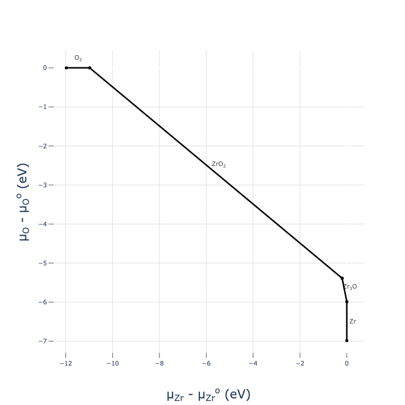
There are a number of ways we can visualize the calculated chemical potential limits. For simply binary systems, we can generate line plots of the chemical potentials:
from pymatgen.analysis.chempot_diagram import ChemicalPotentialDiagram

cpd = ChemicalPotentialDiagram(cpa.intrinsic_phase_diagram.entries)
plot = cpd.get_plot()
plot.show("png", dpi=400)
Because cpd.get_plot() returns a plotly object, it’s almost infinitely customisable using plot.update_scenes() - you can change colours, fonts, axes and even data after it’s been plotted. See the docs for more info.
Beware that because we only generated the relevant competing phases on the Zr-O phase diagram for our ZrO2 host material, we have not calculated all phase in the Zr-O chemical space (just those that are necessary to determine the chemical potential limits of ZrO2), and so these chemical potential diagram plots are only accurate in the vicinity of our host material.
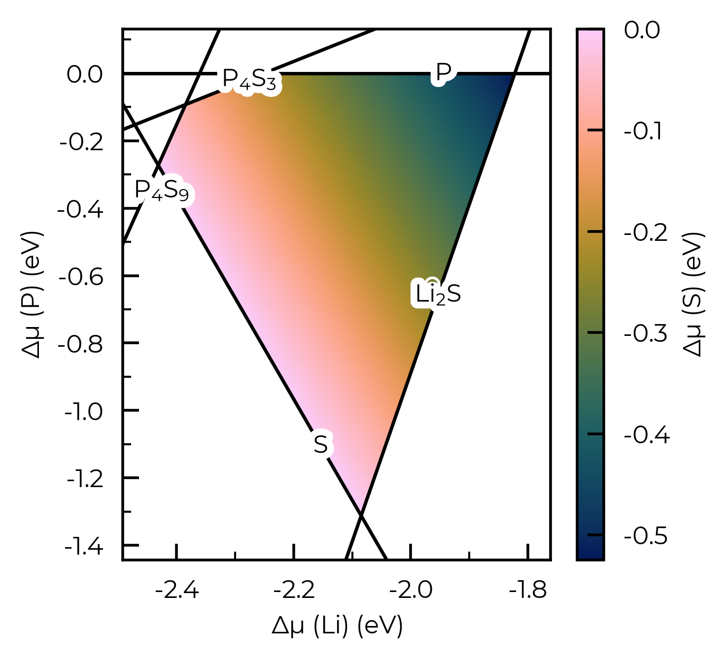
For multinary systems (ternary and above), we can visualise the chemical stability region (range of accessible chemical potentials) as a heatmap plot:
from monty.serialization import loadfn

LiPS4_cpa = loadfn("../tests/data/ChemPotAnalyzers/LiPS4_cpa.json")
plot = LiPS4_cpa.plot_chempot_heatmap()
CompetingPhasesAnalyzer.plot_chempot_heatmap() has many options (some of which are exemplified in the plotting customisation tutorial); see the docstring for more info:
LiPS4_cpa.plot_chempot_heatmap?
Signature:
LiPS4_cpa.plot_chempot_heatmap(
    dependent_element: str | pymatgen.core.periodic_table.Element | None = None,
    fixed_elements: dict[str, float] | None = None,
    bordering_phases: bool = True,
    xlim: tuple[float, float] | None = None,
    ylim: tuple[float, float] | None = None,
    cbar_range: tuple[float, float] | None = None,
    colormap: str | matplotlib.colors.Colormap | None = None,
    padding: float | None = None,
    title: str | bool = False,
    label_positions: bool | dict[str, tuple[float, float]] | list[tuple[float, float]] = True,
    filename: str | pathlib.Path | None = None,
    style_file: str | pathlib.Path | None = None,
    **kwargs,
) -> matplotlib.figure.Figure
Docstring:
Plot a heatmap of the chemical potentials for a multinary system.

In this plot, the ``dependent_element`` chemical potential is plotted
as a heatmap over the stability region of the host composition, as a
function of two other elemental chemical potentials on the x and y
axes.

3-D data is required to plot a 2-D heatmap, and so this function can be
applied as-is for ternary systems, but for higher-dimensional systems
a set of chemical potential constraints must be provided (as
``fixed_elements``) to project the chemical stability region to 3-D;
see the competing phases tutorial:
https://doped.readthedocs.io/en/latest/chemical_potentials_tutorial.html#analysing-and-visualising-the-chemical-potential-limits

Note that due to an issue with ``matplotlib`` ``Stroke`` path effects,
sometimes there can be odd holes in the whitespace around the chemical
formula labels (see: github.com/matplotlib/matplotlib/issues/25669).
This is only the case for ``png`` output, so saving to e.g. ``svg``
or ``pdf`` instead will avoid this issue.

If using the default colour map (``batlow``) in publications, please
consider citing: https://zenodo.org/records/8409685

Tip: https://github.com/frssp/cplapy can be used to generate 3D plots
of chemical stability regions, to show the bordering competing phases
in quaternary systems.

Args:
    dependent_element (str or Element):
        The element for which the chemical potential is plotted as a
        heatmap. If None (default), the last element in the bulk
        composition formula is used (which corresponds to the most
        electronegative element present).
    fixed_elements (dict):
        A dictionary of chemical potentials to fix (in the format:
        ``{element: value}``; e.g. ``{"Li": -2}``) if the chemical
        system is >3-D. Constraining chemical potentials is required for
        multinary systems, in order to reduce the dimensionality to 3-D
        for plotting a 2-D heatmap. For a system with N elements, N-3
        fixed chemical potentials should be specified. If ``None``
        (default), the chemical potentials of the first N-3 elements in
        the bulk composition are fixed to their mean values in the
        stability region (i.e. the centroid of the stability region).
    bordering_phases (bool):
        Whether to plot the competing/secondary phases which border the
        host composition in the chemical potential diagram.
        Default is ``True``.
    xlim (tuple):
        The x-axis limits for the plot. If None (default), the limits
        are set to the minimum and maximum values of the x-axis data,
        with padding equal to ``padding`` (default = 10% of the range).
    ylim (tuple):
        The y-axis limits for the plot. If None (default), the limits
        are set to the minimum and maximum values of the y-axis data,
        with padding equal to ``padding`` (default = 10% of the range).
    cbar_range (tuple):
        The range for the colourbar. If None (default), the range is
        set to the minimum and maximum values of the data.
    colormap (str, matplotlib.colors.Colormap):
        Colormap to use for the heatmap, either as a string (which can
        be a colormap name from https://www.fabiocrameri.ch/colourmaps
        / https://matplotlib.org/stable/users/explain/colors/colormaps)
        or a ``Colormap`` / ``ListedColormap`` object. If ``None``
        (default), uses ``batlow`` from
        https://www.fabiocrameri.ch/colourmaps.

        Append "S" to the colormap name if using a sequential colormap
        from https://www.fabiocrameri.ch/colourmaps.
    padding (float):
        The padding to add to the x and y axis limits. If ``None``
        (default), the padding is set to 10% of the range.
    title (str or bool):
        The title for the plot. If ``False`` (default), no title is
        added. If ``True``, the title is set to the bulk composition
        formula, or if ``str``, the title is set to the provided
        string.
    label_positions (bool, dict or list):
        The positions for the chemical formula line labels. If ``True``
        (default), the labels are placed using a custom ``doped``
        algorithm which attempts to find the best possible positions
        (minimising overlap). If ``False``, no labels are added.
        Alternatively a dictionary can be provided, where the keys are
        the chemical formulae and the values are tuples of
        ``(x_coord, y-offset)`` at which to place the line labels
        (where y-offset is the offset from the line at ``x=x_coord``).
        A list of tuples can also be provided, where the order is
        assumed to match the competing phase lines.
    filename (PathLike):
        The filename to save the plot to. If ``None`` (default), the
        plot is not saved.
    style_file (PathLike):
        Path to a mplstyle file to use for the plot. If ``None``
        (default), uses the default ``doped`` style (from
        ``doped/utils/doped.mplstyle``).
    **kwargs:
        Additional keyword arguments to pass to
        ``ChemicalPotentialDiagram.get_grid()``, such as ``n_points``
        (default = 1000) and ``cartesian`` (default = ``False``).

Returns:
    plt.Figure: The ``matplotlib`` ``Figure`` object.
File:      ~/Packages/doped/doped/chemical_potentials.py
Type:      method
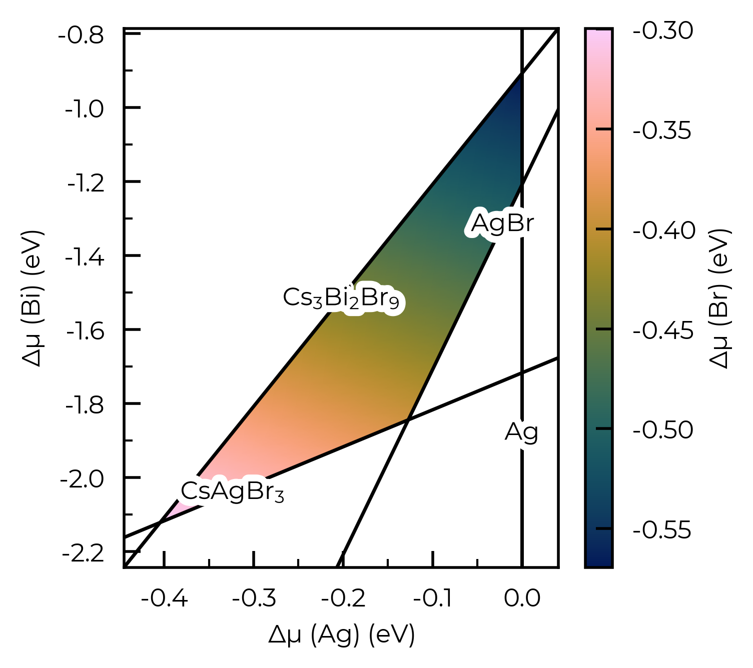
In particular, for systems with more than three elements, we need to specify some chemical potential constraints to reduce the dimensions down to 3-D for plotting in this way. Here is an example for Cs₂AgBiBr₆, where SOC is important for formation energies and thus chemical potentials, as discussed in Guidelines for robust and reproducible point defect simulations in crystals:
# 4-D system:
Cs2AgBiBr6_ncl_cpa = loadfn("../tests/data/ChemPotAnalyzers/Sn_in_Cs2AgBiBr6_ncl_cpa.json")
plot = Cs2AgBiBr6_ncl_cpa.plot_chempot_heatmap(fixed_elements={"Cs": -3.3815})
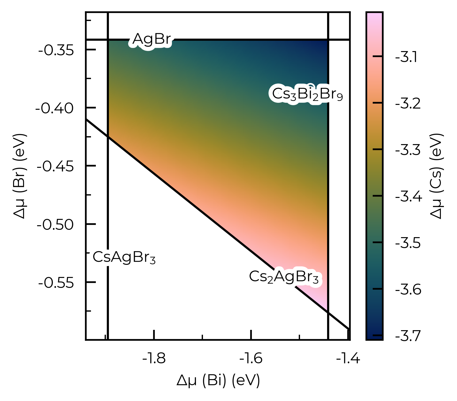
If we do not specify fixed_elements for a >quaternary system, then by default this will be set to match the centroid (mean position) of the stability region, for the first x elements in the system (where x = N - 3 - {any input fixed elements}):
# 4-D system, no fixed elements and Cs as dependent element, so centroid for Ag is used for constraining:
Cs2AgBiBr6_ncl_cpa = loadfn("../tests/data/ChemPotAnalyzers/Sn_in_Cs2AgBiBr6_ncl_cpa.json")
plot = Cs2AgBiBr6_ncl_cpa.plot_chempot_heatmap(dependent_element="Cs")
# the plot_chempot_heatmap() method can also be used with DefectThermodynamics objects:
# DefectThermodynamics.plot_chempot_heatmap()
# or directly with doped.chemical_potentials.plot_chempot_heatmap(chempots, composition="Cu2SiSe3"...)
Chemical potential heatmap plotting requires 3-D data, requiring fixed chemical potential constraints for >ternary systems; such that the number of elements in the chemical system (4) minus the number of fixed chemical potentials (0) must be equal to 3. The following chemical potentials will additionally be constrained to their mean (centroid) values in the chemical stability region: {'Ag': -0.1779}
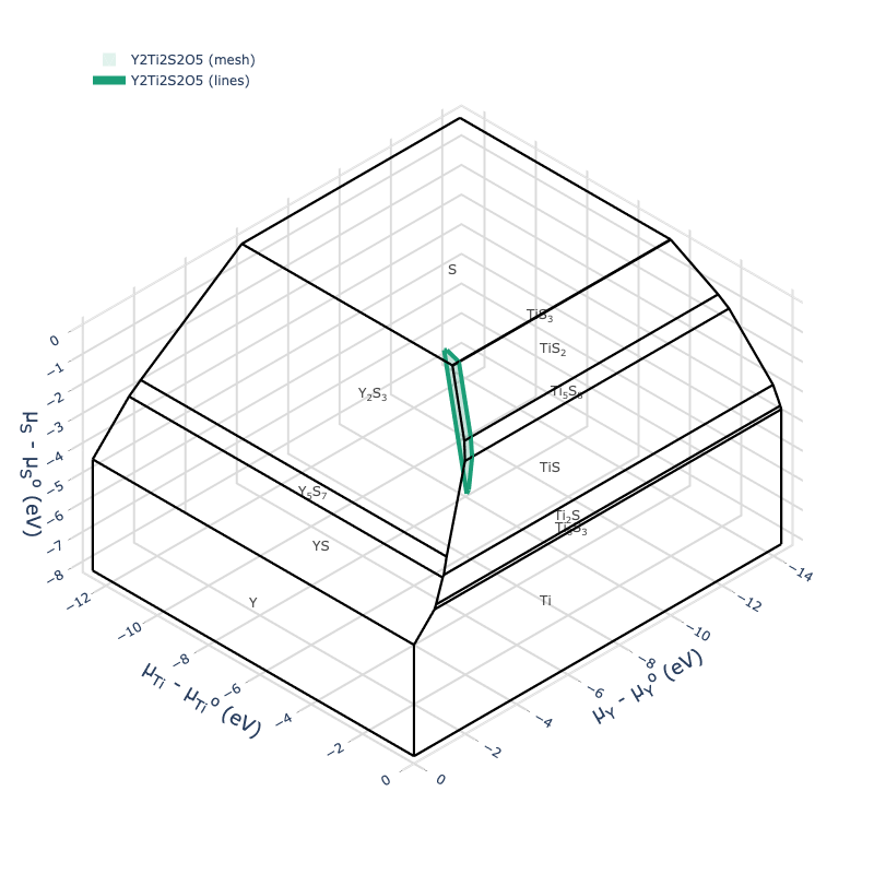
For high-dimensional systems, we can also use the ChemicalPotentialDiagram plotting utilities:
cpd = ChemicalPotentialDiagram(loadfn("YTOS/ytos_phase_diagram.json").entries)
plot = cpd.get_plot(formulas_to_draw=["Y2Ti2S2O5"])
plot.show("png", dpi=400)
We can also get a DataFrame summary of the formation energies of all parsed competing phases:
cpa.get_formation_energy_df() # there is also the prune_polymorphs option here to only show the lowest energy structures for each composition, as well as include_raw_energies, and skip_rounding
| Space Group | Energy above Hull (eV/atom) | Formation Energy (eV/fu) | Formation Energy (eV/atom) | k-points | |
|---|---|---|---|---|---|
| Formula | |||||
| ZrO2 | P2_1/c | 0.000 | -10.975 | -3.658 | 3x3x3 |
| Zr | P6_3/mmc | 0.000 | 0.000 | 0.000 | 9x9x5 |
| O2 | P4/mmm | 0.000 | 0.000 | 0.000 | 2x2x2 |
| Zr3O | R-3c | 0.000 | -5.987 | -1.497 | 5x5x5 |
| ZrO2 | Pbca | 0.008 | -10.951 | -3.650 | 3x3x1 |
| Zr3O | P6_322 | 0.013 | -5.935 | -1.484 | 5x5x5 |
| Zr2O | P312 | 0.019 | -5.729 | -1.910 | 5x5x2 |
| Zr | Ibam | 0.025 | 0.025 | 0.025 | 6x6x6 |
Parsing Extrinsic (Dopant) Competing Phases
If we have generated and calculated competing phases for extrinsic species (i.e. to obtain the chemical potential limits for dopants/extrinsic impurities in our host system), we can parse them in the same manner with CompetingPhasesAnalyzer:
la_cpa = CompetingPhasesAnalyzer(
    composition="ZrO2",  # same host composition
    entries="La_ZrO2_CompetingPhases",  # folder with our competing phase calculations (incl extrinsic)
)
Parsing vaspruns...: 100%|██████████| 11/11 [00:00<00:00, 45.33it/s]
As before, we can get the chemical potential limits in the format required for the DefectThermodynamics plotting and analysis methods using cpa.chempots, which can be easily dumped to a reusable json file for later use:
from monty.serialization import dumpfn, loadfn

dumpfn(la_cpa.chempots, fn="La_ZrO2_CompetingPhases/zro2_la_chempots.json")
la_chemlims = loadfn("La_ZrO2_CompetingPhases/zro2_la_chempots.json")
and we can quickly view the chemical potential limits with chempots_df:
la_cpa.chempots_df
| Zr | O | La | La-Limiting Phase | |
|---|---|---|---|---|
| Limit | ||||
| ZrO2-O2 | -10.97543 | 0.00000 | -9.4630 | La2Zr2O7 |
| Zr3O-ZrO2 | -0.19954 | -5.38794 | -1.3811 | La2Zr2O7 |
CompetingPhasesAnalyzer can likewise parse and compute the chemical potential limits with multiple extrinsic species present.
Summarising & Saving Results for Publication
Often we may want to summarise the results of our competing phases and chemical potential limit calculations, to include in the SI of journal articles or theses to aid open-science and reproducibility, or for quick data sharing, or for use with other codes. There are a number of simple methods for achieving this with the CompetingPhasesAnalyzer class and properties.
Save Formation Energies and Chemical Potentials to File
As shown above, we can get DataFrame summaries of the formation energies of our calculated competing phases, and the computed chemical potential limits using CompetingPhasesAnalyzer.get_formation_energy_df() and CompetingPhasesAnalyzer.chempots_df respectively. These DataFrames can be saved to file with the DataFrame.to_csv() method, which we can then import as a table in Microsoft Word or convert to LaTeX format with www.tablesgenerator.com/latex_tables:
# e.g. here as an example I get the formation energy dataframe, include the DFT energies,
# remove the 'eV/atom' columns, and only include the lowest energy polymorph for each phase
form_energy_df = cpa.get_formation_energy_df(prune_polymorphs=True, include_raw_energies=True)
form_energy_df = form_energy_df.drop(columns=[col for col in form_energy_df.columns if "eV/atom" in col])
form_energy_df
| Space Group | Formation Energy (eV/fu) | DFT Energy (eV/fu) | k-points | |
|---|---|---|---|---|
| Formula | ||||
| ZrO2 | P2_1/c | -10.975 | -34.832 | 3x3x3 |
| Zr | P6_3/mmc | 0.000 | -9.844 | 9x9x5 |
| O2 | P4/mmm | 0.000 | -14.013 | 2x2x2 |
| Zr3O | R-3c | -5.987 | -42.524 | 5x5x5 |
| Zr2O | P312 | -5.729 | -32.423 | 5x5x2 |
form_energy_df.to_csv("ZrO2_Competing_Phase_Formation_Energies.csv") # save to csv file
We could also do the same with CompetingPhasesAnalyzer.chempots_df.
Print Formation Energies as a LaTeX Table
We also provide the to_LaTeX_table method to directly convert the parsed formation energies into a LaTeX table, either as a one- or two-column table; ordered alphabetially or in descending order of energies:
cpa.to_LaTeX_table()  # we can then copy and paste this into LaTeX
# this also comes with `prune_polymorphs` (True by default) and `splits` options, see docstring for info
\begin{table}[h]
\centering
\caption{Formation energies per formula unit ($\Delta E_f$) of \ce{ZrO2} and all competing phases, with k-meshes used in calculations. Only the lowest energy polymorphs are included.}
\label{tab:competing_phase_formation_energies}
\begin{tabular}{ccccc}
\hline
Formula & Space Group & E$_{\textrm{Hull}}$ (eV/atom) & k-mesh & $\Delta E_f$ (eV/fu) \\ \hline
\ce{ZrO2} & P2$_{1}$/c & 0.000 & 3$\times$3$\times$3 & -10.975 \\
\ce{Zr} & P6$_{3}$/mmc & 0.000 & 9$\times$9$\times$5 & 0.000 \\
\ce{O2} & P4/mmm & 0.000 & 2$\times$2$\times$2 & 0.000 \\
\ce{Zr3O} & R$\overline{3}$c & 0.000 & 5$\times$5$\times$5 & -5.987 \\
\ce{Zr2O} & P312 & 0.019 & 5$\times$5$\times$2 & -5.729 \\
\hline
\end{tabular}
\end{table}
Note
The table does not use booktabs by default but you can change the horizontal lines (hline) to
toprule, midrule and bottomrule to get the desired style effect. The output also relies on using the
\ce{} command from the mhchem LaTeX package to get the correct formatting for the chemical formulae.
Save to JSON
As with all the doped objects, we can also save the CompetingPhasesAnalyzer object to JSON with:
from monty.serialization import dumpfn
dumpfn(cpa, "ZrO2_cpa.json")
And reload with loadfn:
from monty.serialization import loadfn
reloaded_cpa = loadfn("ZrO2_cpa.json")
reloaded_cpa.chempots_df
| Zr | O | |
|---|---|---|
| Limit | ||
| ZrO2-O2 | -10.97543 | 0.00000 |
| Zr3O-ZrO2 | -0.19954 | -5.38794 |
Chemical Systems with Many Polymorphs
For many elements and compounds, there are many metastable allotropes/polymorphs on the Materials Project database (and often in experimental reality). Depending on our energy_above_hull setting with CompetingPhases, this can result in a large number of competing phases to calculate and consider, which can be time- and resource-intensive.
It is only the lowest energy allotrope/polymorph of a given composition which can border the host composition on the phase diagram (and thus determine chemical potential limits), and so if we have some insights on which phases we expect to be the ground-states, we can use this to reduce the number of competing phases that need to be calculated. If the Materials Project (MP) energies – queried automatically within the CompetingPhases class initialisation – were perfectly accurate, then we could always just use energy_above_hull=0 and only consider the MP ground-states. However we know that this is not the case for many/most systems, and so we typically use a non-zero energy_above_hull error range to ensure we don’t miss out on any true ground-states.
Often, we do not have a priori knowledge of the ground-state phase (according to our computational setup / temperature conditions), and so this issue of dealing with many competing phase calculations is unavoidable. In other cases, however, we may know what the ground-state phase is for our computational setup based on previous projects/calculations, literature, collaborators or otherwise, or can use experimental data if available and appropriate. Some examples of this are shown below.
Known Ground-State Phases
Let’s say we want to compute the chemical stability region for Sb₂S₃ (e.g. as performed in this defect study):
from doped.chemical_potentials import CompetingPhases

Sb2S3_cp = CompetingPhases(composition="Sb2S3")
print(f"Number of competing phases: {len(Sb2S3_cp)}")

# number of competing phases by composition:
from collections import defaultdict
comp_entries_dict = defaultdict(list)
for e in Sb2S3_cp.entries:
    comp_entries_dict[e.composition.reduced_formula].append(e)

for comp, entries in comp_entries_dict.items():
    print(f"{comp}: {len(entries)} entries to consider")
Here we can see that with the default energy_above_hull MP energy tolerance of 0.05 eV/atom, we have 2 potential competing phases for Sb₂S₃, 2 for elemental Sb, and 20 for elemental S. This is a result of the highly allotropic nature of sulfur, which has many low-energy metastable structures.
In this case, we know from our previous work that the ground-state phase of Sb₂S₃ is the Pnma phase with MP energy-above-hull of 0 eV/atom, and the ground-state phase of S is the mp-77 phase (close-packed S8 molecules), when using hybrid DFT (HSE06). Thus we can reduce to only these phases for these compositions to dramatically reduce the number of competing phases that need to be calculated:
# reduce to only the ground-state phases for Sb2S3 and S:
all_MP_entries = Sb2S3_cp.entries
reduced_MP_entries = []
for entry in all_MP_entries:
    if entry.name == "Sb2S3":
        if "Pnma" in entry.data["doped_name"]:  # only Pnma phase
            reduced_MP_entries.append(entry)
    elif entry.name == "S":
        if "mp-77" in entry.data["material_id"]:  # only mp-77 phase
            reduced_MP_entries.append(entry)
    else:
        reduced_MP_entries.append(entry)
len(reduced_MP_entries) # 1 Sb2S3 phase, 1 S phase, 2 Sb phases
Update the CompetingPhases object to only include this reduced set of entries:
Sb2S3_cp.entries = reduced_MP_entries
kpoint_convergence_sets = Sb2S3_cp.write_kpoint_convergence_files(
    output_path="Sb2S3_CompetingPhases",
    # potcar_spec=True  # uncomment to run on Colab!
)
!ls Sb2S3_CompetingPhases
We have recorded some known ground-states/room-temperature phases for a selection of common elements and compounds with several allotropes/polymorphs, in the docs/known_MP_ground_states.md file, which can be used in a similar manner as shown above to reduce the number of competing phases that need to be calculated.
One can set the optional parameter expected_polymorphs to True (False by default) to automatically prune the set of candidate competing phases to only the expected ground-state/room-temperature polymorphs for each composition (if the data is available in the doped/utils/known_MP_ground_states.yaml file, otherwise does not prune), as well as the lowest energy-above-hull entry according to the MP database (if not already one of the expected polymorphs).
For example with Sb₂S₃:
from doped.chemical_potentials import CompetingPhases

Sb2S3_cp = CompetingPhases(composition="Sb2S3", expected_polymorphs=True)
print(f"Number of competing phases: {len(Sb2S3_cp)}")

# number of competing phases by composition:
from collections import defaultdict
comp_entries_dict = defaultdict(list)
for e in Sb2S3_cp.entries:
    comp_entries_dict[e.composition.reduced_formula].append(e)

for comp, entries in comp_entries_dict.items():
    print(f"{comp}: {len(entries)} entries to consider")
Using expected_polymorphs=True in this case reduces the number of competing phases to consider from 24 to 5, reducing to the known R-3m ground-state for Sb, and the expected room-temperature and moderate-to-high-temperature (~400 - ~1000 K) ground-states for S (close-packed S8 molecules, and gas-phase S8).
Note that, as mentioned in docs/known_MP_ground_states.md, gas-phase S2 (disulfur) is the dominant sulfur vapour phase at high temperatures (T ~> 1000 K). The corresponding molecular phase can be generated as a molecule-in-a-box structure with the doped.chemical_potentials.make_molecule_in_a_box function, or molecule-in-a-box entry with the doped.chemical_potentials.make_molecular_entry function, if desired (i.e. if considering temperature conditions ~>1000 K and including finite-temperature effects such as vibrational free energies and ideal gas entropy contributions):
!rm -r Sb2S3_CompetingPhases  # remove previous outputs
# add gas-phase S2:
from doped.chemical_potentials import make_molecular_entry

# input elemental-S entry to ``make_molecular_entry`` to generate a gas-phase S2 entry:
gas_phase_S2 = make_molecular_entry(Sb2S3_cp.entries_dict["S_Fddd_EaH_0"])
Sb2S3_cp.entries.append(gas_phase_S2)  # S_mmm_EaH_0 = molecular phase
relaxation_sets = Sb2S3_cp.write_relaxation_files(
    output_path="Sb2S3_CompetingPhases",
    # potcar_spec=True  # uncomment to run on Colab!
)
!ls Sb2S3_CompetingPhases
See the docs/known_MP_ground_states.md file for more details on known/expected ground-state polymorphs. If you know of other cases with many low-energy polymorphs on the MP database, but known ground-state phases, please submit a pull request to add to this list!
Experimentally-Known Ground-State Phases
In some other cases, we can try using experimental data to reduce the number of competing phases that need to be calculated. For instance, if we are confident that only the experimentally-observed phase(s) are relevant for our system, computational setup and temperature conditions, then we could reduce the set of candidate phases to only those with matching ICSD IDs:
Sb2S3_cp = CompetingPhases(composition="Sb2S3")
print(f"Number of competing phases: {len(Sb2S3_cp)}")
The IDs of matching experimental database entries are stored in the ComputedEntry.data["summary"]["database_IDs"] attribute of the doped competing phase entries:
Sb2S3_cp.entries[1].data["summary"]["database_IDs"]
Let’s reduce our set of candidate entries here to only those which have at least one matching experimental database ID:
reduced_MP_entries = [e for e in Sb2S3_cp.entries if e.data["summary"]["database_IDs"]]
print(f"Number of competing phases with at least one matching experimental ID: {len(reduced_MP_entries)}")

Sb2S3_cp.entries = reduced_MP_entries
from collections import defaultdict
comp_entries_dict = defaultdict(list)
for e in Sb2S3_cp.entries:
    comp_entries_dict[e.composition.reduced_formula].append(e)

for comp, entries in comp_entries_dict.items():
    print(f"{comp}: {len(entries)} entries to consider")
Here this only partially reduces our set of candidate competing phases, mostly because the large range of metastable allotropes of elemental sulfur on the MP database is a reflection of the large range of experimentally-observed sulfur phases. For an alternative example – TiO₂ – we can see that this pruning to only experimentally-observed phases has a larger effect:
TiO2_cp = CompetingPhases(composition="TiO2")
print(f"Number of competing phases: {len(TiO2_cp)}")
reduced_MP_entries = [e for e in TiO2_cp.entries if e.data["summary"]["database_IDs"]]
print(f"Number of competing phases with at least one matching experimental ID: {len(reduced_MP_entries)}")
Warning
In some cases, pruning to only ‘experimentally-observed’ phases may not be totally accurate, potentially due to MP-mislabelling, or due to dynamic averaging effects in experimental XRD missing ground-state distortions (e.g. octahedral tilting and distortions in perovskites, site disorder etc – see this example in AgBiS₂) – and/or experimental structures corresponding to high-temperature polymorphs.
As mentioned in the tip near the top of this tutorial, in some cases if our accuracy requirement is less stringent (e.g. for high-throughput screening), we can set energy_above_hull=0 to only consider the MP ground-state phase for each relevant composition – recomputing this phase with our chosen computational setup is typically still a significant improvement in accuracy over simply taking MP energies and chemical potentials as-is.