Tips & Tricks

The development philosophy behind doped has been to try build a powerful, efficient and flexible code for managing and analysing solid-state defect calculations, having reasonable defaults (that work well for the majority of materials/defects) but with full flexibility for the user to customise the workflow to their specific needs/system.

Note

Much of the advice for defect calculations given here and elsewhere centres on the message that, while we try to provide some rough general rules-of-thumb for reasonable choices in the calculation workflow (based on the literature and our experience), there is no substitute for the user’s own judgement. Defect behaviour can be incredibly system-dependent, and so it is always important to question and consider the choices and approximations made in the workflow (such as supercell choice, charge state ranges, interstitial site pruning, MAGMOM initialisation etc.) in the context of your specific host system.

Interstitials

As described in the YouTube defect calculation tutorial, our recommended workflow for calculating interstitial defects is to first generate the set of candidate interstitial sites for your structure using DefectsGenerator (which uses Voronoi tessellation for this, see note below), and then perform Gamma-point-only relaxations (using vasp_gam) for each charge state of the generated interstitial candidates, and then pruning some of the candidate sites based on the criteria below. Typically the easiest way to do this is to follow the workflow shown in the defect generation tutorial, and then run the ShakeNBreak vasp_gam relaxations for the Unperturbed and Bond_Distortion_0.0%/Rattled directories of each charge state. Alternatively you can generate the vasp_gam relaxation input files by setting vasp_gam = True in DefectsSet.write_files().

We can then compare the energies of these trial relaxations, and remove candidates that either:

• Are very high energy (~>1 eV above the lowest energy site for each charge state), and so are unlikely to form.

• Relax to the same final structure/energy as other interstitial sites (despite different initial positions) in each charge state, and so are unnecessary to calculate. This can happen due to interstitial migration within the relaxation calculation, from an unfavourable higher energy site, to a lower energy one. Typically if the energy from the test vasp_gam relaxations are within a couple meV of eachother, this is the case.

Tip

As with many steps in the defect calculation workflow, these are only rough general rules-of-thumb and you should always critically consider the validity of these choices in the context of your specific system (for example, considering the charge-state dependence of the interstitial site formation energies here).

Note

As mentioned above, by default Voronoi tessellation is used to generate the candidate interstitial sites in doped. We have consistently found this approach to be the most robust in identifying all stable/low-energy interstitial sites across a wide variety of materials and chemistries. A nice discussion of this is given in Kononov et al. J. Phys.: Condens. Matter 2023.

As with all aspects of the calculation workflow however, interstitial site generation is highly flexible, and you can explicitly specify the interstitial sites to generate using the interstitial_coords (for instance, if you only want to investigate one specific known interstitial site, or input a list of candidate sites generated from a different algorithm), and/or customise the generation algorithm via interstitial_gen_kwargs, both of which are input parameters for the DefectsGenerator class; see the API documentation for more details.

Charge-density based approaches for interstitial site generation can be useful in some cases and often output less candidate sites, but we have found that these are primarily suited to ionic materials (and with fully-ionised defect charge states) where electrostatics primarily govern the energetics. In many systems (particularly those with some presence of (ionic-)covalent bonding) where orbital hybridisation plays a role, this approach can often miss the ground-state interstitial site(s). .. If you are highly limited with computational resources and are working with (relatively simple) ionic compound(s), this approach may be worth considering.

Difficult Structural Relaxations

If defect supercell relaxations do not converge after multiple continuation calculations (i.e. cp-ing CONTCAR to POSCAR and resubmitting the job), this is likely due to small residual forces causing the local optimisation algorithm to struggle to find a solution, an error in the underlying calculation and/or extreme forces.

• If the calculation outputs show that the relaxation is proceeding fine, without any errors, just not converging to completion, then it suggests that the structure relaxation is bouncing around a narrow region of the potential energy surface. Here, the gradient-based geometry optimiser is struggling to converge.

  • Often (but not always) this indicates that the structure may be stuck around a saddle point or shallow local minimum on the potential energy surface (PES), so it’s important to make sure that you have performed structure-searching (PES scanning) with ShakeNBreak (SnB) to avoid this. You may want to try ‘rattling’ the structure to break symmetry in case this is an issue, as detailed in this part of the SnB docs.

  • Alternatively (if you have already performed `SnB` structure-seaerching), convergence of the forces can be aided by:

  • Switching the ionic relaxation algorithm back and forth (i.e. change IBRION to 1 or 3 and back).

  • Reducing the ionic step width (e.g. change POTIM to 0.02 in the INCAR)

  • Switching the electronic minimisation algorithm (e.g. change ALGO to All), if electronic convergence seems to be causing issues.

  • Tightening/reducing the electronic convergence criterion (e.g. change EDIFF to 1e-7)

• If instead the calculation is crashing due to an error and/or extreme forces, a common culprit is the EDWAV error in the output file, which can often be avoided by reducing NCORE and/or KPAR. If this doesn’t fix it, switching the electronic minimisation algorithm (e.g. change ALGO to All) can sometimes help.

  • If some relaxations are still not converging after multiple continuations, you should check the calculation output files to see if this requires fixing. Often this may require changing a specific INCAR setting, and using the updated setting(s) for any other relaxations that are also struggling to converge.

ShakeNBreak

For tips on the ShakeNBreak part of the defect calculation workflow, please refer to the ShakeNBreak documentation.

Layered / Low-Dimensional Materials

Layered and low-dimensional materials can add some additional complications when performing defect analysis in these systems. One point is that typically such lower symmetry materials exhibit higher rates of energy-lowering defect reconstructions (e.g. 4-electron negative-U centres in Sb₂Se₃), as a result of having more complex energy landscapes.

Another is that often the application of charge correction schemes to supercell calculations with layered materials may require some fine-tuning for converged results. To illustrate, for Sb₂Si₂Te₆ ( a promising layered thermoelectric material), when parsing the intrinsic defects, the -3 charge antimony vacancy (v_Sb-3) gave this warning:

Estimated error in the Kumagai (eFNV) charge correction for defect v_Sb_-3 is 0.067 eV (i.e. which is
greater than the `error_tolerance`: 0.050 eV). You may want to check the accuracy of the correction by
plotting the site potential differences (using `defect_entry.get_kumagai_correction()` with `plot=True`).
Large errors are often due to unstable or shallow defect charge states (which can't be accurately modelled
with the supercell approach). If this error is not acceptable, you may need to use a larger supercell
for more accurate energies.

Following the advice in the warning, we use defect_entry.get_kumagai_correction(plot=True) to plot the site potential differences for the defect supercell (which is used to obtain the eFNV (Kumagai-Oba) anisotropic charge correction):

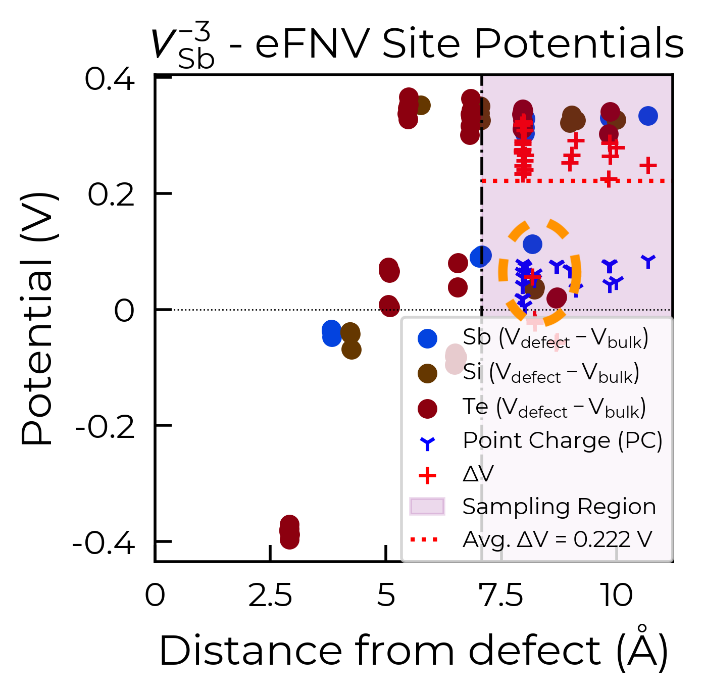
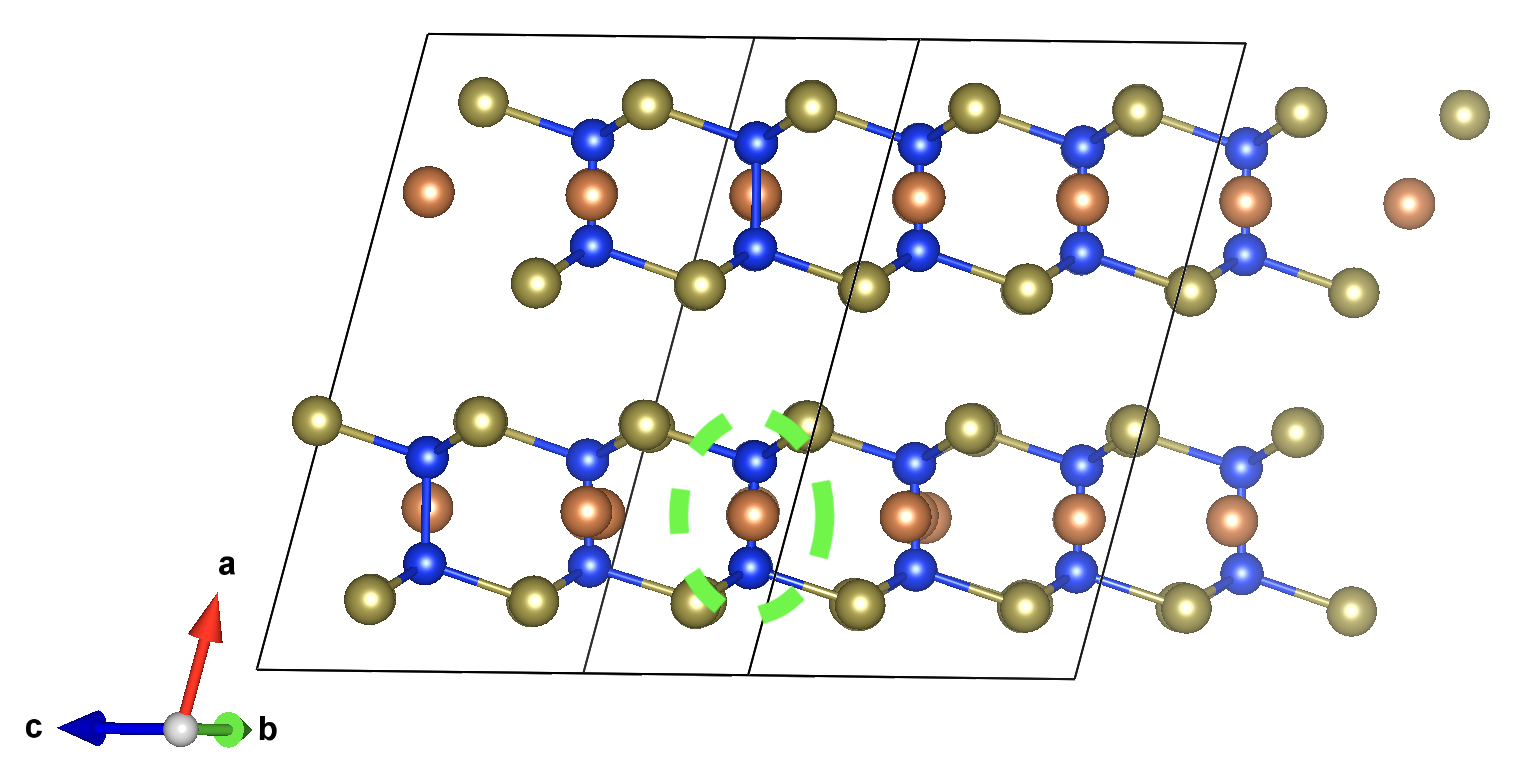
From the eFNV plot, we can see that there appears to be two distinct sets of site potentials, with one curving up from ~-0.4 V to ~0.1 V, and another mostly constant set at ~0.3 V. We can understand this by considering the structure of our defect (shown on the right), where the location of the Sb vacancy (hidden by the projection along the plane) is circled in green – we can see the displacement of the Sb atoms on either side.

Due to the layered structure, the charge and strain associated with the defect is mostly confined to the defective layer, while that of the layer away from the defect mostly experiences the typical long-range electostatic potential of the defect charge. The same behaviour can be seen for h-BN in the original eFNV paper (Figure 4d). This means that our usual default of using the Wigner-Seitz radius to determine the sampling region is not as good, as it’s including sites in the defective layer (circled in orange) which are causing the variance in the potential offset (ΔV) and thus the error in the charge correction.

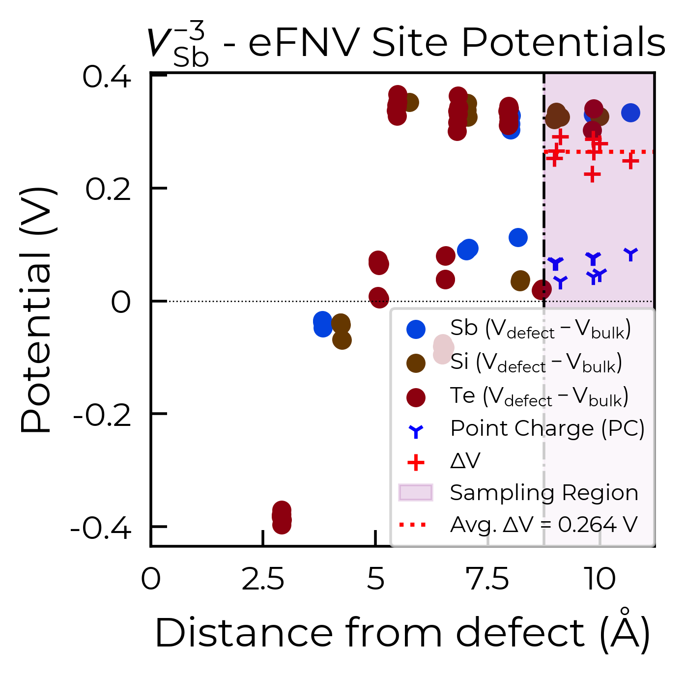
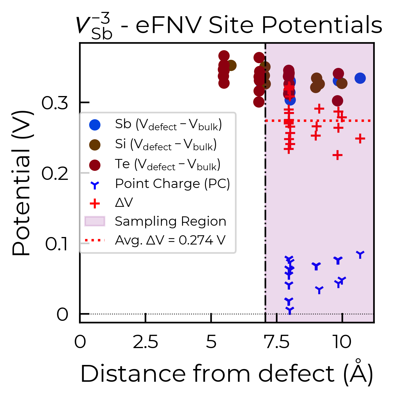
To fix this, we can use the optional defect_region_radius or excluded_indices parameters in get_kumagai_correction, to exclude those points from the sampling. For defect_region_radius, we can just set this to 8.75 Å here to avoid those sites in the defective layer. Often it may not be so simple to exclude the intra-layer sites in this way (depending on the supercell), and so alternatively we can use excluded_indices for more fine-grained control. As we can see in the structure image above, the a lattice vector is aligned along the inter-layer direction, so we can determine the intra-layer sites using the fractional coordinates of the defect site along a:

# get indices of sites within 0.2 fractional coordinates along a of the defect site
sites_in_layer = [
    i for i, site in enumerate(defect_entry.defect_supercell)
    if abs(site.frac_coords[0] - defect_entry.defect_supercell_site.frac_coords[0]) < 0.2
]
correction, fig =  dp.defect_dict["v_Sb-3"].get_kumagai_correction(
    excluded_indices=sites_in_layer, plot=True
)  # note that this updates the DefectEntry.corrections value, so the updated correction
# is used in later formation energy / concentration calculations

Below are the two resulting charge correction plots (using defect_region_radius on the left, and excluded_indices on the right):

Note

Have any tips for users from using doped? Please share it with the developers and we’ll add them here!