Advanced Defect Analysis

Here we describe some more targeted analysis you can do for your defect calculations parsed with doped (including comparing the relaxed configurations for different initial interstitial positions, structure & bond length analysis of defects, and plotting/analysis of the defect charge corrections), which may be useful for in certain cases.

Defect-Induced Site Displacements (Strain)

Using the DefectEntry.plot_site_displacements() method, we can analyse the displacements of atoms around the defect site (i.e. defect-induced local strain) during geometry relaxation.

%matplotlib inline
from monty.serialization import loadfn
CdTe_defects_thermo = loadfn("CdTe/CdTe_thermo_wout_meta.json")  # load our DefectThermodynamics object

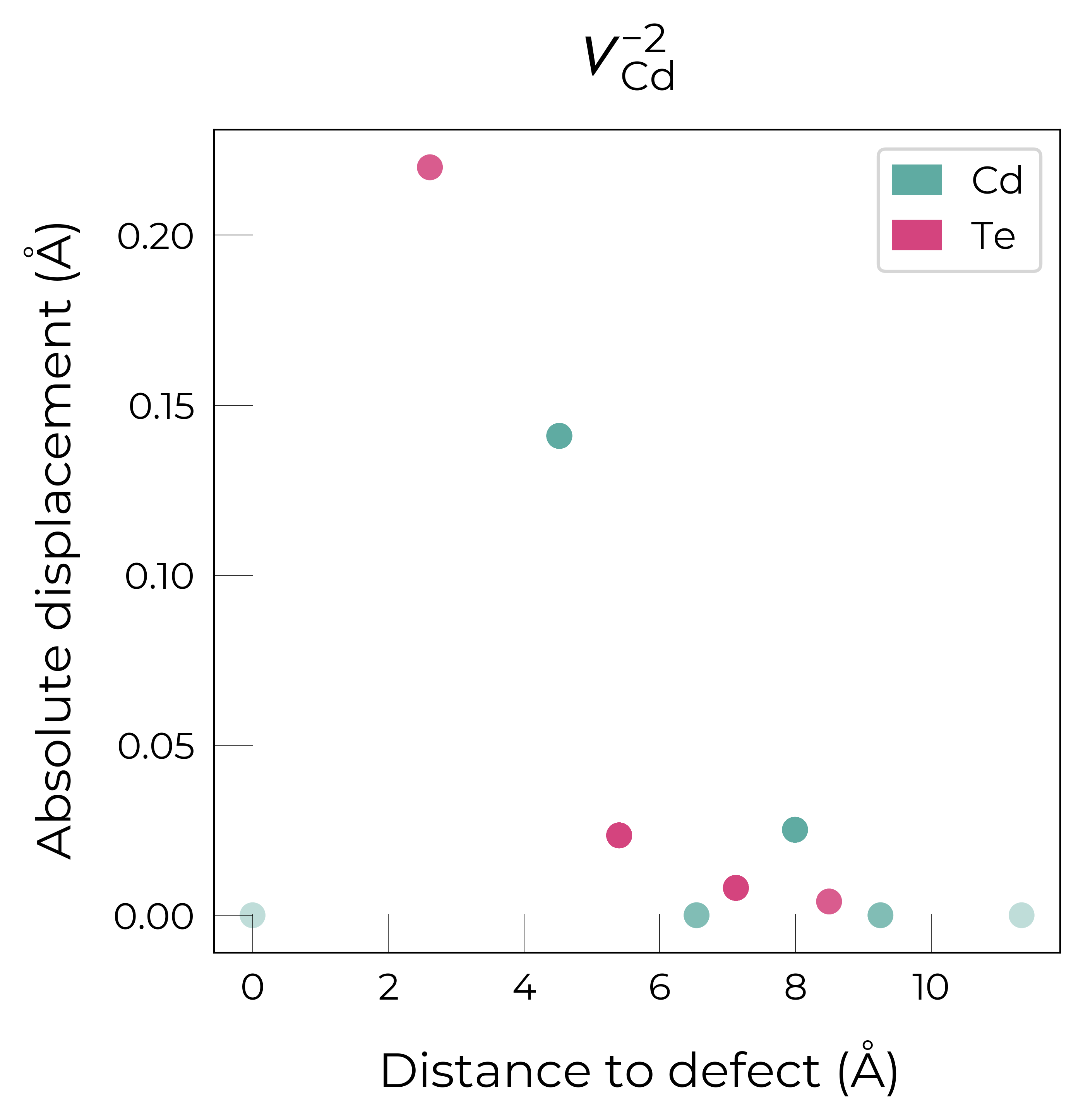
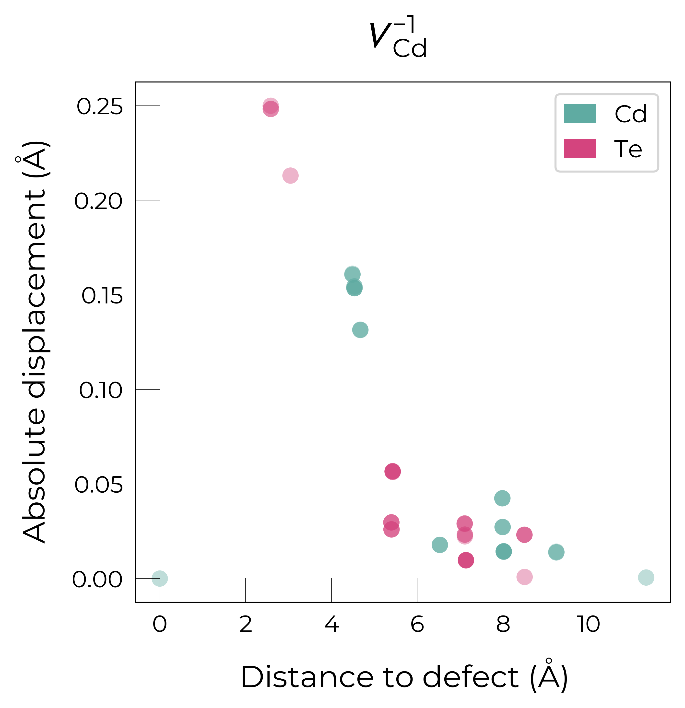
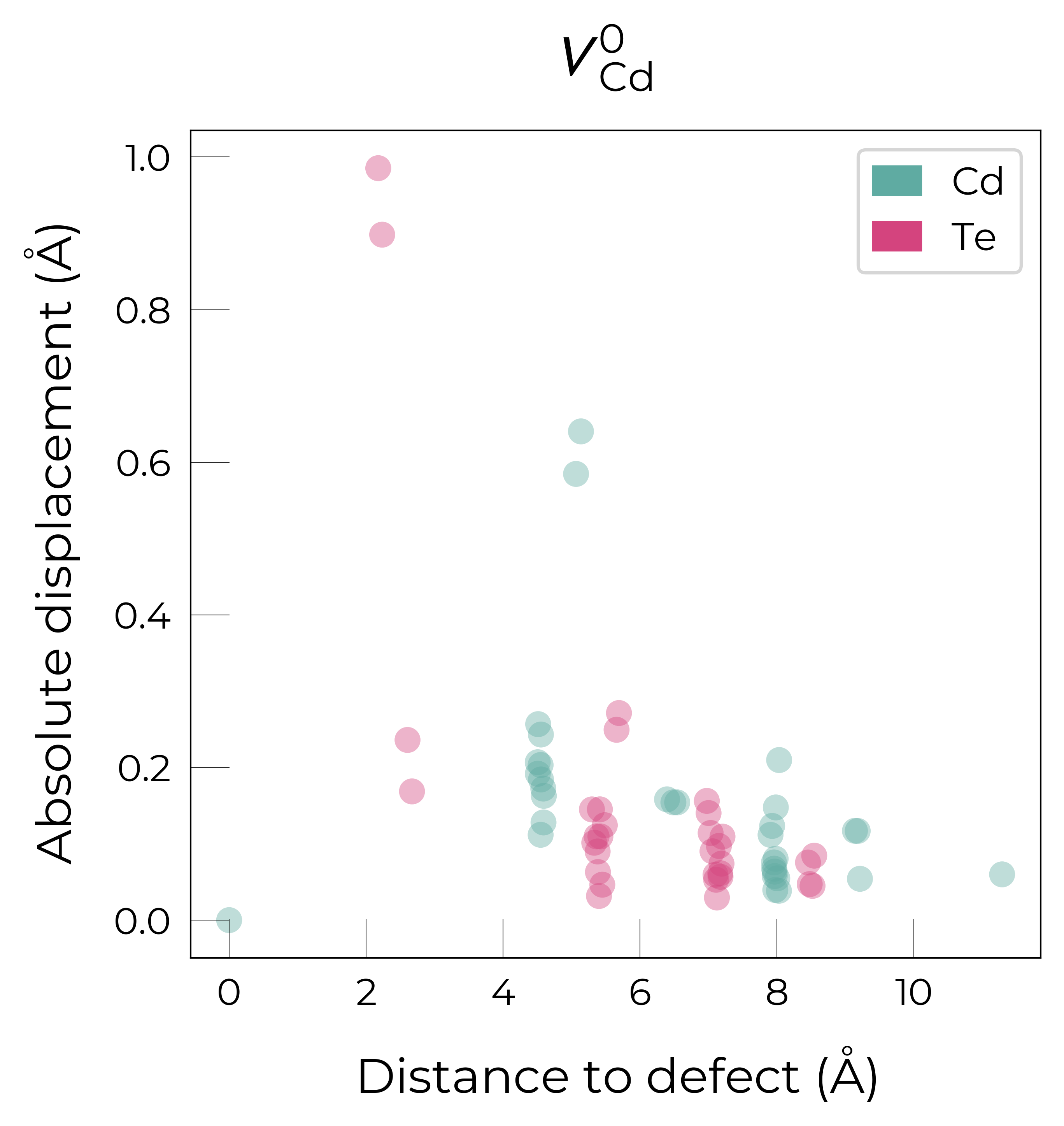
Let’s look at the displacements of atoms around the Cd vacancy in CdTe, and how this changes with charge state:

from doped.utils.plotting import _format_defect_name

v_Cd_entries = [entry for entry in CdTe_defects_thermo.defect_entries if "v_Cd" in entry.name]
for defect_entry in v_Cd_entries:
    fig = defect_entry.plot_site_displacements(separated_by_direction=False)
    fig.suptitle(_format_defect_name(defect_entry.name, include_site_info_in_name=False), 
                 fontsize=18)

Separated by direction:

from doped.utils.plotting import _format_defect_name

v_Cd_entries = [entry for entry in CdTe_defects_thermo.defect_entries if "v_Cd" in entry.name]
for defect_entry in v_Cd_entries:
    fig = defect_entry.plot_site_displacements()
    fig.suptitle(_format_defect_name(defect_entry.name, include_site_info_in_name=False), 
                 y=1.2, fontsize=22)

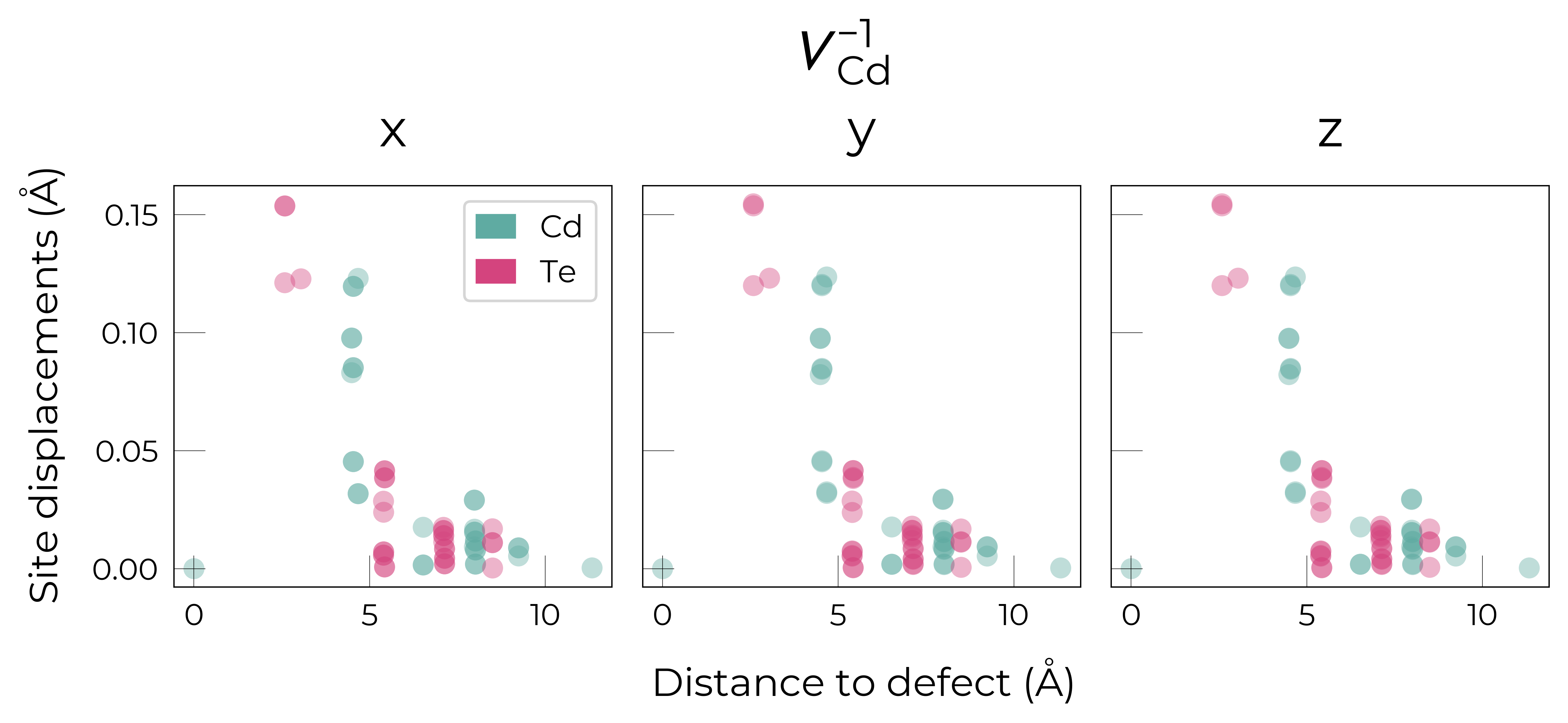
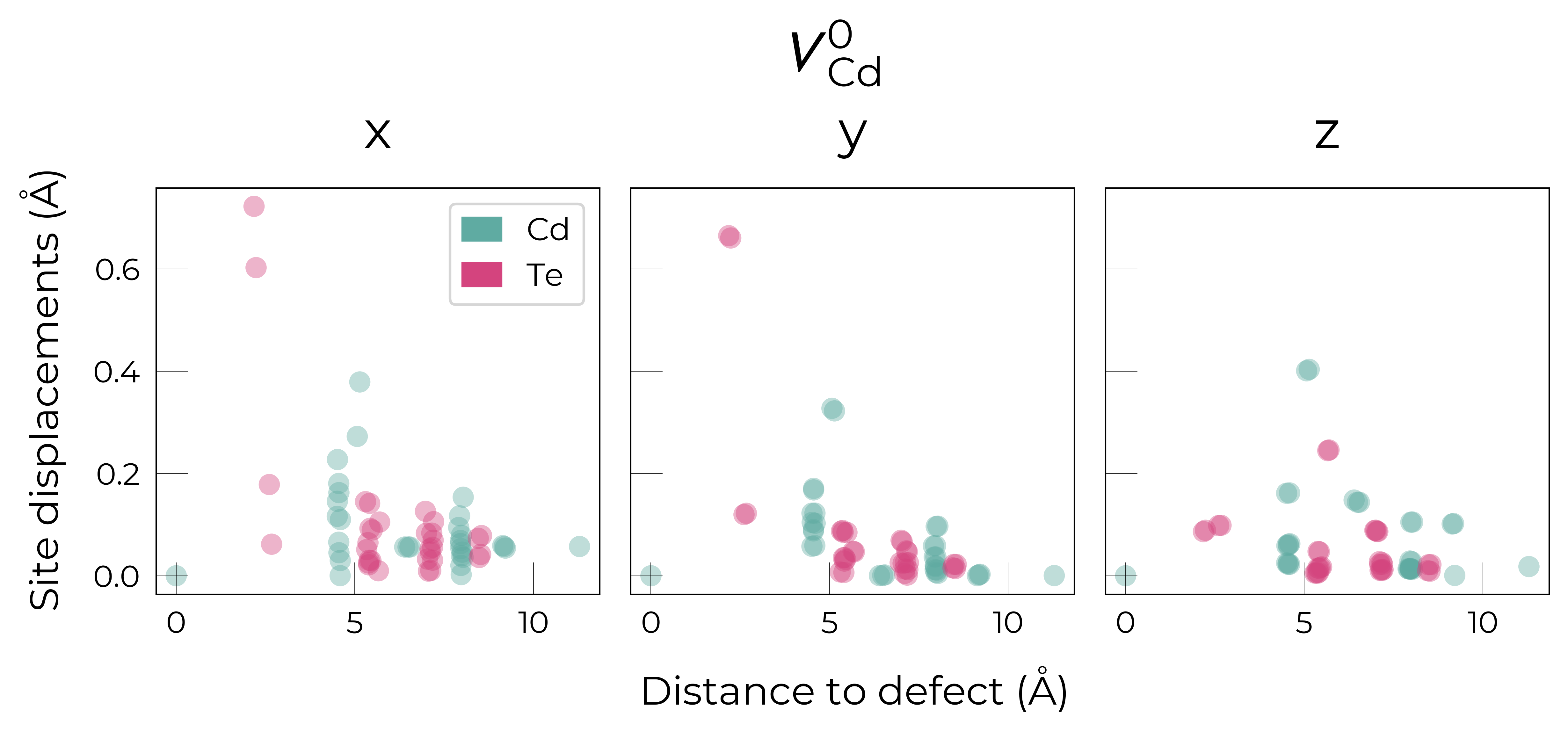
Here we see that \(V_{Cd}^{-2}\) has isotropic (symmetric) displacements of atoms around the vacancy site in the x/y/z directions, which makes sense as it adopts a tetrahedral (Td) geometry (as shown in the get_symmetries_and_degeneracies output below and discussed in detail in this paper). As expected, we see an exponential tail-off in the site displacement magnitudes as we move away from the defect, and it is the Te nearest neighbours which are most strongly perturbed.

For \(V_{Cd}^{-1}\), we have a Jahn-Teller-distorted \(C_{3v}\) geometry where a neighbouring Te atom displaces along the [111] direction away from the vacancy site (while the other Te atoms displace away from the vacancy but by a smaller degree), while for \(V_{Cd}^{0}\), we have a \(C_{2v}\) geometry where two neighbouring Te displace significantly toward eachother (~1 Å) and form a dimer bond, while the other two Te move a smaller distance away (~0.2 Å) as seen in the displacement plots.

from doped.thermodynamics import DefectThermodynamics
v_Cd_thermo = DefectThermodynamics(v_Cd_entries)
v_Cd_thermo.get_symmetries_and_degeneracies()

	Defect	q	Site_Symm	Defect_Symm	g_Orient	g_Spin	g_Total	Mult
0	v_Cd	-2	Td	Td	1.0	1	1.0	1.0
1	v_Cd	-1	Td	C3v	4.0	2	8.0	1.0
2	v_Cd	0	Td	C2v	6.0	1	6.0	1.0

The high symmetry of \(V_{Cd}^{-2}\) is evident from the displacement plots above, where it looks like there are much fewer atoms in the plots, however this is just because we have many symmetry-equivalent atoms in this case and so we end up with many overlapping points (and so much less distinct points). Then for \(C_{3v}\) \(V_{Cd}^{-1}\) we have more distinct sites appearing, and then more so for the lower-symmetry \(C_{2v}\) \(V_{Cd}^{0}\) structure.

Processing Cdᵢ vasp_gam calculations to see which site is favoured

import os
from doped.analysis import DefectParser

bulk_path = "CdTe/CdTe_bulk/vasp_gam/"  # path to bulk (defect-free) supercell calculation
dielectric = 9.13  # calculated dielectric constant, required for computing defect charge corrections
Cd_i_dict = {}  # Keep dictionary of parsed defect entries

for i in os.listdir("CdTe"):
    if 'Cd_i' in i:
        Cd_i_dict[i] = DefectParser.from_paths(
            defect_path=f"CdTe/{i}/vasp_gam/", bulk_path=bulk_path, dielectric=dielectric).defect_entry

for defect_name, defect_entry in Cd_i_dict.items():
    print(f"Name: {defect_name}; Raw Supercell Energy: {defect_entry.get_ediff():.3f} eV")
    # note this energy is just the energy difference of the bulk and defect supercells (including 
    # finite-size charge corrections if any – none here as they're neutral defects), without Fermi
    # level or chemical potential terms (though these are constant for the same defect & charge)

Name: Cd_i_Td_Cd2.83_0; Raw Supercell Energy: 0.592 eV
Name: Cd_i_C3v_0; Raw Supercell Energy: 0.728 eV
Name: Cd_i_Td_Te2.83_0; Raw Supercell Energy: 0.728 eV

Here we see that the Cd-coordinated interstitial site is the lowest energy for neutral cadmium interstitials here!

Note

The energies here do not yet account for the chemical potentials, which are included later in the post-processing workflow (as shown earlier in this notebook). However, the chemical potential energy correction is the same for each charge state or site, for a given defect (e.g. Cd_i here) - hence the relative energies are still meaningful here.

Here we see that Cd_i_C3v_0 and Cd_i_Td_Te2.83_0 have equal final energies (rounded to 1 meV/atom) suggesting they have relaxed to the same final structure (despite different initial interstitial positions). Let’s use StructureMatcher and local_env to double-check:

# Here we use the pymatgen StructureMatcher class to compare the relaxed structures of neutral Cd_i:
from pymatgen.analysis.structure_matcher import StructureMatcher
sm = StructureMatcher()
print("Are Cd_i_Td_Cd2.83_0 and Cd_i_C3v_0 final structures the same?:",
      sm.fit(Cd_i_dict['Cd_i_Td_Cd2.83_0'].defect_supercell, Cd_i_dict['Cd_i_C3v_0'].defect_supercell))
print("Are Cd_i_C3v_0 and Cd_i_Td_Te2.83_0 final structures the same?:",
      sm.fit(Cd_i_dict['Cd_i_C3v_0'].defect_supercell, Cd_i_dict['Cd_i_Td_Te2.83_0'].defect_supercell))

Are Cd_i_Td_Cd2.83_0 and Cd_i_C3v_0 final structures the same?: False
Are Cd_i_C3v_0 and Cd_i_Td_Te2.83_0 final structures the same?: True

# we can perform further defect structural analysis with these functions:
from pymatgen.analysis.local_env import CrystalNN
import numpy as np

for key, defect_entry in Cd_i_dict.items():
    # get defect site index in structure: (needed for CrystalNN)
    for i, site in enumerate(defect_entry.defect_supercell.sites):
        if np.isclose(site.frac_coords, defect_entry.defect_supercell_site.frac_coords).all():
            isite = i  # site index, starting from 0

    crystalNN = CrystalNN()
    struct = defect_entry.defect_supercell
    struct.add_oxidation_state_by_guess()
    print("Local order parameters (i.e. resemblence to given structural motif): ",
          crystalNN.get_local_order_parameters(struct, isite))
    print("Nearest-neighbour dictionary: ",
          crystalNN.get_cn_dict(struct, isite))

    bond_lengths = []  # Bond Lengths?
    for i in crystalNN.get_nn_info(struct, isite):
        bond_lengths.append({'Element': i['site'].specie.as_dict()['element'],
                             'Distance': f"{i['site'].distance(struct[isite]):.3f}"})
    print("Bond-lengths (in Angstrom) to nearest neighbours: ", bond_lengths, "\n")

Local order parameters (i.e. resemblence to given structural motif):  None
Nearest-neighbour dictionary:  {'Te0+': 6, 'Cd0+': 4}
Bond-lengths (in Angstrom) to nearest neighbours:  [{'Element': 'Te', 'Distance': '3.298'}, {'Element': 'Te', 'Distance': '3.298'}, {'Element': 'Te', 'Distance': '3.298'}, {'Element': 'Te', 'Distance': '3.298'}, {'Element': 'Te', 'Distance': '3.298'}, {'Element': 'Te', 'Distance': '3.298'}, {'Element': 'Cd', 'Distance': '3.007'}, {'Element': 'Cd', 'Distance': '3.007'}, {'Element': 'Cd', 'Distance': '3.007'}, {'Element': 'Cd', 'Distance': '3.007'}] 

Local order parameters (i.e. resemblence to given structural motif):  {'square co-planar': 0.08049643519922586, 'tetrahedral': 0.9999935468913711, 'rectangular see-saw-like': 0.007133072179242341, 'see-saw-like': 0.23547633536015408, 'trigonal pyramidal': 0.24644908542744104}
Nearest-neighbour dictionary:  {'Te0+': 4}
Bond-lengths (in Angstrom) to nearest neighbours:  [{'Element': 'Te', 'Distance': '2.911'}, {'Element': 'Te', 'Distance': '2.911'}, {'Element': 'Te', 'Distance': '2.911'}, {'Element': 'Te', 'Distance': '2.911'}] 

Local order parameters (i.e. resemblence to given structural motif):  {'square co-planar': 0.07996844283674677, 'tetrahedral': 0.9999999999971609, 'rectangular see-saw-like': 0.0070246315480141, 'see-saw-like': 0.23425410407519495, 'trigonal pyramidal': 0.2452100857961308}
Nearest-neighbour dictionary:  {'Te0+': 4}
Bond-lengths (in Angstrom) to nearest neighbours:  [{'Element': 'Te', 'Distance': '2.911'}, {'Element': 'Te', 'Distance': '2.911'}, {'Element': 'Te', 'Distance': '2.911'}, {'Element': 'Te', 'Distance': '2.911'}] 

Here we see the structural similarity of “Cd_i_C3v_0” and “Cd_i_Td_Te2.83_0”, showing that they have indeed relaxed to the same structure. This means we only need to continue with one of these for the more expensive vasp_std and vasp_ncl calculations with our full k-point mesh.

Note

If you want to do this coordination environment analysis with a vacancy, you may have to introduce a fake atom at the vacancy position, in order to create a pymatgen Site object, to then use with CrystalNN. For example:

from doped.thermodynamics import DefectThermodynamics
v_Cd_thermo = DefectThermodynamics(
    [entry for entry in CdTe_example_thermo.defect_entries if "v_Cd" in entry.name], 
    chempots=CdTe_example_thermo.chempots
)  # only Cd vacancy defects

from pymatgen.analysis.local_env import CrystalNN
from doped.thermodynamics import bold_print

for defect_entry in v_Cd_thermo.defect_entries:
    bold_print(f"{defect_entry.name}, Charge State: {defect_entry.charge_state}")
    crystalNN = CrystalNN(distance_cutoffs=None, x_diff_weight=0.0, porous_adjustment=False, search_cutoff=5)
    struct = defect_entry.defect_supercell.copy()
    struct.append('U', defect_entry.defect_supercell_site.frac_coords) # Add a fake element
    isite = len(struct.sites) - 1 # Starts counting from zero!

    print("Local order parameters (i.e. resemblance to given structural motif): ",
          crystalNN.get_local_order_parameters(struct, isite))
    print("Nearest-neighbour dictionary: ", crystalNN.get_cn_dict(struct, isite))

    bond_lengths = []  # Bond Lengths?
    for i in crystalNN.get_nn_info(struct,isite):
        bond_lengths.append({'Element': i['site'].specie.as_dict()['element'],
                             'Distance': f"{i['site'].distance(struct[isite]):.3f}"})
    print("Bond-lengths (in Angstrom) to nearest neighbours: ",bond_lengths,"\n")

v_Cd_-2, Charge State: -2
Local order parameters (i.e. resemblance to given structural motif):  {'square co-planar': 0.07996848894580866, 'tetrahedral': 0.999999999996243, 'rectangular see-saw-like': 0.007024644113827354, 'see-saw-like': 0.23425369905750856, 'trigonal pyramidal': 0.24520967518806777}
Nearest-neighbour dictionary:  {'Te': 4}
Bond-lengths (in Angstrom) to nearest neighbours:  [{'Element': 'Te', 'Distance': '2.613'}, {'Element': 'Te', 'Distance': '2.613'}, {'Element': 'Te', 'Distance': '2.613'}, {'Element': 'Te', 'Distance': '2.613'}] 

v_Cd_-1, Charge State: -1
Local order parameters (i.e. resemblance to given structural motif):  {'square co-planar': 0.08955199275710107, 'tetrahedral': 0.9980437792997895, 'rectangular see-saw-like': 0.00914205834683717, 'see-saw-like': 0.2561471898083992, 'trigonal pyramidal': 0.2673736880526364}
Nearest-neighbour dictionary:  {'Te': 4}
Bond-lengths (in Angstrom) to nearest neighbours:  [{'Element': 'Te', 'Distance': '2.585'}, {'Element': 'Te', 'Distance': '2.587'}, {'Element': 'Te', 'Distance': '2.587'}, {'Element': 'Te', 'Distance': '3.046'}] 

v_Cd_0, Charge State: 0
Local order parameters (i.e. resemblance to given structural motif):  {'square co-planar': 0.1554382566688805, 'tetrahedral': 0.7810051379511412, 'rectangular see-saw-like': 0.052869064285435134, 'see-saw-like': 0.22758740109965894, 'trigonal pyramidal': 0.23528866099223875}
Nearest-neighbour dictionary:  {'Te': 4}
Bond-lengths (in Angstrom) to nearest neighbours:  [{'Element': 'Te', 'Distance': '2.178'}, {'Element': 'Te', 'Distance': '2.605'}, {'Element': 'Te', 'Distance': '2.235'}, {'Element': 'Te', 'Distance': '2.671'}]