Defect Calculation Parsing

For parsing defect calculation results with doped, we need the following VASP output files from our bulk and defect supercell calculations:

• vasprun.xml(.gz)

• Either:

  • OUTCAR(.gz), if using the Kumagai-Oba (eFNV) charge correction scheme (compatible with isotropic or anisotropic (non-cubic) dielectric constants; recommended), or

  • LOCPOT(.gz), if using the Freysoldt (FNV) charge correction scheme (isotropic dielectric screening only).

Note that doped can read the compressed versions of these files (.gz/.xz/.bz/.lzma), so we can do e.g. gzip OUTCAR to reduce the file sizes when downloading and storing these files on our local system.

To quickly compress these output files on our HPC, we can run the following from our top-level folder containing the defect directories (e.g. Te_i_Te2.83_+2 etc):

(change OUTCAR to LOCPOT if using the FNV isotropic charge correction), and then download the files to the relevant folders by running the following from our local system:

changing [remote_machine] and [path to doped folders] accordingly.

Example: CdTe Defect Calculations

In this example, we parse some defect calculations for CdTe. In this case, these defects weren’t initially generated with doped, but this is fine, as doped can parse the results and automatically determine the defect type and site from the relaxed structure.

Note

If you want to use the example outputs shown in this parsing tutorial, you can do so by cloning the doped GitHub repository and following the dope_parsing_example.ipynb Jupyter notebook. In this case, you will witness some extra warnings during parsing due to some mismatching tags in the bulk/defect outputs – purposely included for testing.

from doped.analysis import DefectsParser
%matplotlib inline 

bulk_path = "CdTe/CdTe_bulk/vasp_ncl"  # path to our bulk supercell calculation
dielectric = 9.13  # dielectric constant (this can be a single number (isotropic), or a 3x1 array or 3x3 matrix (anisotropic))

dp = DefectsParser("CdTe", dielectric=dielectric)  # dielectric needed for charge corrections

Parsing v_Cd_-2/vasp_ncl: 100%|██████████| 7/7 [00:56<00:00,  6.74s/it]               analysis.py:1051: UserWarning: Warning(s) encountered when parsing Int_Te_3_Unperturbed_1 at CdTe/Int_Te_3_Unperturbed_1/vasp_ncl:
There are mismatching INCAR tags for your bulk and defect calculations which are likely to cause severe errors in the parsed results (energies). Found the following differences:
(in the format: (INCAR tag, value in bulk calculation, value in defect calculation)):
[('ADDGRID', True, False)]
The same INCAR settings should be used in both calculations for these tags which can affect energies!

Parsing v_Cd_-2/vasp_ncl: 100%|██████████| 7/7 [00:56<00:00,  8.14s/it]

DefectsParser uses multiprocessing by default to speed up parsing when we have many defect supercell calculations to parse. As described in its docstring shown below, it automatically searches the supplied output_path for the bulk and defect supercell calculation folders, then automatically determines the defect types, sites (from the relaxed structures) and charge states.

It also checks that appropriate INCAR, KPOINTS, POTCAR settings have been used, and will warn you if it detects any differences that could affect the defect formation energies, as shown in the example above with the mismatching ADDGRID tag (here we have manually checked that this choice did not affect the defect formation energies).

DefectsParser?

Init signature:
DefectsParser(
    output_path: str = '.',
    dielectric: Union[float, int, numpy.ndarray, NoneType] = None,
    subfolder: Optional[str] = None,
    bulk_path: Optional[str] = None,
    skip_corrections: bool = False,
    error_tolerance: float = 0.05,
    bulk_bandgap_path: Optional[str] = None,
    processes: Optional[int] = None,
    json_filename: Union[str, bool, NoneType] = None,
)
Docstring:      <no docstring>
Init docstring:
A class for rapidly parsing multiple VASP defect supercell calculations
for a given host (bulk) material.

Loops over calculation directories in `output_path` (likely the same
`output_path` used with `DefectsSet` for file generation in `doped.vasp`)
and parses the defect calculations into a dictionary of:
{defect_name: DefectEntry}, where the defect_name is set to the defect
calculation folder name (_if it is a recognised defect name_), else it is
set to the default `doped` name for that defect. By default, searches for
folders in `output_path` with `subfolder` containing `vasprun.xml(.gz)`
files, and tries to parse them as `DefectEntry`s.

By default, tries to use multiprocessing to speed up defect parsing, which
can be controlled with the `processes` parameter.

Defect charge states are automatically determined from the defect calculation
outputs if `POTCAR`s are set up with `pymatgen` (see docs Installation page),
or if that fails, using the defect folder name (must end in "_+X" or "_-X"
where +/-X is the defect charge state).

Uses the (single) `DefectParser` class to parse the individual defect
calculations. Note that the bulk and defect supercells should have the same
definitions/basis sets (for site-matching and finite-size charge corrections
to work appropriately).

Args:
    output_path (str):
        Path to the output directory containing the defect calculation
        folders (likely the same `output_path` used with `DefectsSet` for
        file generation in `doped.vasp`). Default = current directory.
    dielectric (float or int or 3x1 matrix or 3x3 matrix):
        Ionic + static contributions to the dielectric constant. If not provided,
        charge corrections cannot be computed and so `skip_corrections` will be
        set to true.
    subfolder (str):
        Name of subfolder(s) within each defect calculation folder (in the
        `output_path` directory) containing the VASP calculation files to
        parse (e.g. `vasp_ncl`, `vasp_std`, `vasp_gam` etc.). If not
        specified, `doped` checks first for `vasp_ncl`, `vasp_std`, `vasp_gam`
        subfolders with calculation outputs (`vasprun.xml(.gz)` files) and uses
        the highest level VASP type (ncl > std > gam) found as `subfolder`,
        otherwise uses the defect calculation folder itself with no subfolder
        (set `subfolder = "."` to enforce this).
    bulk_path (str):
        Path to bulk supercell reference calculation folder. If not specified,
        searches for folder with name "X_bulk" in the `output_path` directory
        (matching the default `doped` name for the bulk supercell reference folder).
    skip_corrections (bool):
        Whether to skip the calculation and application of finite-size charge
        corrections to the defect energies (not recommended in most cases).
        Default = False.
    error_tolerance (float):
        If the estimated error in any charge correction is greater than
        this value (in eV), then a warning is raised. (default: 0.05 eV)
    bulk_bandgap_path (str):
        Path to bulk OUTCAR file for determining the band gap. If the VBM/CBM
        occur at reciprocal space points not included in the bulk supercell
        calculation, you should use this tag to point to a bulk bandstructure
        calculation instead. Alternatively, you can edit/add the "gap" and "vbm"
        entries in DefectParser.defect_entry.calculation_metadata to match the
        correct (eigen)values.
        If None, will calculate "gap"/"vbm" using the outputs at:
        DefectParser.defect_entry.calculation_metadata["bulk_path"]
    processes (int):
        Number of processes to use for multiprocessing for expedited parsing.
        If not set, defaults to one less than the number of CPUs available.
    json_filename (str):
        Filename to save the parsed defect entries dict (`DefectsParser.defect_dict`)
        to in `output_path`, to avoid having to re-parse defects when later analysing
        further and aiding calculation provenance. Can be reloaded using the `loadfn`
        function from `monty.serialization` as shown in the docs, or
        `DefectPhaseDiagram.from_json()`. If None (default), set as
        "{Chemical Formula}_defect_dict.json" where {Chemical Formula} is the
        chemical formula of the host material. If False, no json file is saved.

Attributes:
    defect_dict (dict):
        Dictionary of parsed defect calculations in the format:
        {"defect_name": DefectEntry}) where the defect_name is set to the
        defect calculation folder name (_if it is a recognised defect name_),
        else it is set to the default `doped` name for that defect.
File:           ~/Library/CloudStorage/OneDrive-ImperialCollegeLondon/Bread/Projects/Packages/doped/doped/analysis.py
Type:           type
Subclasses:     

doped automatically attempts to perform the appropriate finite-size charge correction method for each defect, based on the supplied dielectric constant and calculation outputs, and will warn you if any required outputs are missing.

Additionally, the DefectsParser class automatically checks the consistency and estimated error of the defect finite-size charge correction, and will warn you if the estimated error is above error_tolerance (50 meV by default). As shown later in the Charge Corrections section, we can directly visualise the finite-size charge correction plots (showing how they are being computed) easily with doped, which is recommended if any of these warnings about the charge correction accuracy are printed.

With our dictionary of parsed defect entries, we can then query some of the defect-specific results, such as the finite-size charge corrections, the defect site, and energy (without accounting for chemical potentials yet):

for name, defect_entry in dp.defect_dict.items():
    print(f"{name}:")
    if defect_entry.charge_state != 0:  # no charge correction for neutral defects
        print(f"Charge = {defect_entry.charge_state:+} with finite-size charge correction: {list(defect_entry.corrections.values())[0]:+.2f} eV")
    print(f"Supercell site: {defect_entry.defect_supercell_site.frac_coords.round(3)}\n")

Int_Te_3_1:
Charge = +1 with finite-size charge correction: +0.30 eV
Supercell site: [0.801 0.166 0.699]

v_Cd_0:
Supercell site: [0.5 0.5 0.5]

Te_Cd_+1:
Charge = +1 with finite-size charge correction: +0.24 eV
Supercell site: [0.475 0.475 0.525]

Int_Te_3_Unperturbed_1:
Charge = +1 with finite-size charge correction: +0.30 eV
Supercell site: [0.716 0.283 0.871]

Int_Te_3_2:
Charge = +2 with finite-size charge correction: +0.90 eV
Supercell site: [0.835 0.944 0.698]

v_Cd_-1:
Charge = -1 with finite-size charge correction: +0.23 eV
Supercell site: [0. 0. 0.]

v_Cd_-2:
Charge = -2 with finite-size charge correction: +0.74 eV
Supercell site: [0. 0. 0.]

As mentioned in the defect generation tutorial, we can save doped outputs to JSON files and then share or reload them later on, without needing to re-run the parsing steps above. Here we save our parsed defect entries using the dumpfn function from monty.serialization:

from monty.serialization import dumpfn, loadfn
dumpfn(dp.defect_dict, "CdTe_defect_dict.json")  # save parsed defect entries to file

# we can then reload these parsed defect entries from file at any later point with:
CdTe_defect_dict = loadfn("CdTe_defect_dict.json")

Defect Formation Energy / Transition Level Diagrams

Tip

Defect formation energy (a.k.a. transition level diagrams) are one of the key results from a computational defect study, giving us a lot of information on the defect thermodynamics and electronic behaviour.

Important

To calculate and plot the defect formation energies, we generate a DefectPhaseDiagram object, which can be created using the analysis.dpd_from_defect_dict() function, which takes a dictionary of parsed defect entries and outputs the DefectPhaseDiagram:

# generate DefectPhaseDiagram object, with which we can plot/tabulate formation energies, calculate charge transition levels etc:
from doped.analysis import dpd_from_defect_dict
CdTe_example_dpd = dpd_from_defect_dict(dp.defect_dict)
dumpfn(CdTe_example_dpd, "CdTe_example_dpd.json")  # save parsed DefectPhaseDiagram to file, so we don't need to regenerate it later

To calculate and plot defect formation energies, we need to know the chemical potentials of the elements in the system (see the YouTube defects tutorial for more details on this). The workflow for computing and analysing the chemical potentials is described in the Competing Phases tutorial, and here we have already done this for our CdTe system, so we can just load the results from the JSON file here:

# load CdTe parsed chemical potentials (needed to compute the defect formation energies)
CdTe_chempots = loadfn("CdTe/CdTe_chempots.json")

print(CdTe_chempots)

{'facets': {'Cd-CdTe': {'Cd': -1.01586484, 'Te': -5.7220097228125}, 'CdTe-Te': {'Cd': -2.2671822228125, 'Te': -4.47069234}}, 'elemental_refs': {'Te': -4.47069234, 'Cd': -1.01586484}, 'facets_wrt_el_refs': {'Cd-CdTe': {'Cd': 0.0, 'Te': -1.2513173828125002}, 'CdTe-Te': {'Cd': -1.2513173828125, 'Te': 0.0}}}

Some of the advantages of parsing / manipulating your chemical potential calculations this way, is that:

• You can quickly loop through different points in chemical potential space (i.e. phase diagram facets), rather than typing out the chemical potentials obtained from a different method / manually.

• doped automatically determines the chemical potentials with respect to elemental references (i.e. chemical potentials are zero in their standard states (by definition), rather than VASP/DFT energies). This is the facets_wrt_el_refs entry in the CdTe_chempots dict in the cell above.

• doped can then optionally print the corresponding phase diagram facet / chemical potential limit and the formal chemical potentials of the elements at that point, above the formation energy plot, as shown in the next cell.

Alternatively, you can directly feed in pre-calculated chemical potentials to doped, see below for this.

Basic formation energy plot:

from doped import plotting
def_plot = plotting.formation_energy_plot(
    CdTe_example_dpd,
    CdTe_chempots,
    facets=["CdTe-Te"],
)

There are a lot of options for making the formation energy plot prettier:

# you can run this cell to see the possible arguments for this function:
plotting.formation_energy_plot?
# or go to the python API documentation for this function:
# https://doped.readthedocs.io/en/latest/doped.plotting.html#doped.plotting.formation_energy_plot

Signature:
plotting.formation_energy_plot(
    defect_phase_diagram,
    chempots: Optional[Dict] = None,
    facets: Union[List, str, NoneType] = None,
    el_refs: Optional[Dict] = None,
    chempot_table: bool = True,
    all_entries: Union[bool, str] = False,
    style_file: Optional[str] = None,
    xlim: Optional[Tuple] = None,
    ylim: Optional[Tuple] = None,
    fermi_level: Optional[float] = None,
    colormap: Union[str, matplotlib.colors.Colormap] = 'Dark2',
    auto_labels: bool = False,
    filename: Optional[str] = None,
)
Docstring:
Produce a defect formation energy vs Fermi level plot (a.k.a. a defect
formation energy / transition level diagram). Returns the Matplotlib Figure
object to allow further plot customisation.

Args:
    defect_phase_diagram (DefectPhaseDiagram):
        DefectPhaseDiagram for which to plot defect formation energies
        (typically created from analysis.dpd_from_defect_dict).
    chempots (dict):
        Dictionary of chemical potentials to use for calculating the defect
        formation energies. This can have the form of
        {"facets": [{'facet': [chempot_dict]}]} (the format generated by
        doped's chemical potential parsing functions (see tutorials)) and
        facet(s) (chemical potential limit(s)) to plot can be chosen using
        `facets`, or a dictionary of **DFT**/absolute chemical potentials
        (not formal chemical potentials!), in the format:
        {element symbol: chemical potential} - if manually specifying
        chemical potentials this way, you can set the el_refs option with
        the DFT reference energies of the elemental phases in order to show
        the formal (relative) chemical potentials above the plot.
        (Default: None)
    facets (list, str):
        A string or list of facet(s) (chemical potential limit(s)) for which
        to plot the defect formation energies, corresponding to 'facet' in
        {"facets": [{'facet': [chempot_dict]}]} (the format generated by
        doped's chemical potential parsing functions (see tutorials)). If
        not specified, will plot for each facet in `chempots`. (Default: None)
    el_refs (dict):
        Dictionary of elemental reference energies for the chemical potentials
        in the format:
        {element symbol: reference energy} (to determine the formal chemical
        potentials, when chempots has been manually specified as
        {element symbol: chemical potential}). Unnecessary if chempots is
        provided in format generated by doped (see tutorials).
        (Default: None)
    chempot_table (bool):
        Whether to print the chemical potential table above the plot.
        (Default: True)
    all_entries (bool, str):
        Whether to plot the formation energy lines of _all_ defect entries,
        rather than the default of showing only the equilibrium states at each
        Fermi level position (traditional). If instead set to "faded", will plot
        the equilibrium states in bold, and all unstable states in faded grey
        (Default: False)
    style_file (str):
        Path to a mplstyle file to use for the plot. If None (default), uses
        the default doped style (from doped/utils/doped.mplstyle).
    xlim:
        Tuple (min,max) giving the range of the x-axis (Fermi level). May want
        to set manually when including transition level labels, to avoid crossing
        the axes. Default is to plot from -0.3 to +0.3 eV above the band gap.
    ylim:
        Tuple (min,max) giving the range for the y-axis (formation energy). May
        want to set manually when including transition level labels, to avoid
        crossing the axes. Default is from 0 to just above the maximum formation
        energy value in the band gap.
    fermi_level (float):
        If set, plots a dashed vertical line at this Fermi level value, typically
        used to indicate the equilibrium Fermi level position (e.g. calculated
        with py-sc-fermi). (Default: None)
    colormap (str, matplotlib.colors.Colormap):
        Colormap to use for the formation energy lines, either as a string (i.e.
        name from https://matplotlib.org/stable/users/explain/colors/colormaps.html)
        or a Colormap / ListedColormap object. (default: "Dark2")
    auto_labels (bool):
        Whether to automatically label the transition levels with their charge
        states. If there are many transition levels, this can be quite ugly.
        (Default: False)
    filename (str): Filename to save the plot to. (Default: None (not saved))

Returns:
    Matplotlib Figure object, or list of Figure objects if multiple facets
    chosen.
File:      ~/Library/CloudStorage/OneDrive-ImperialCollegeLondon/Bread/Projects/Packages/doped/doped/plotting.py
Type:      function

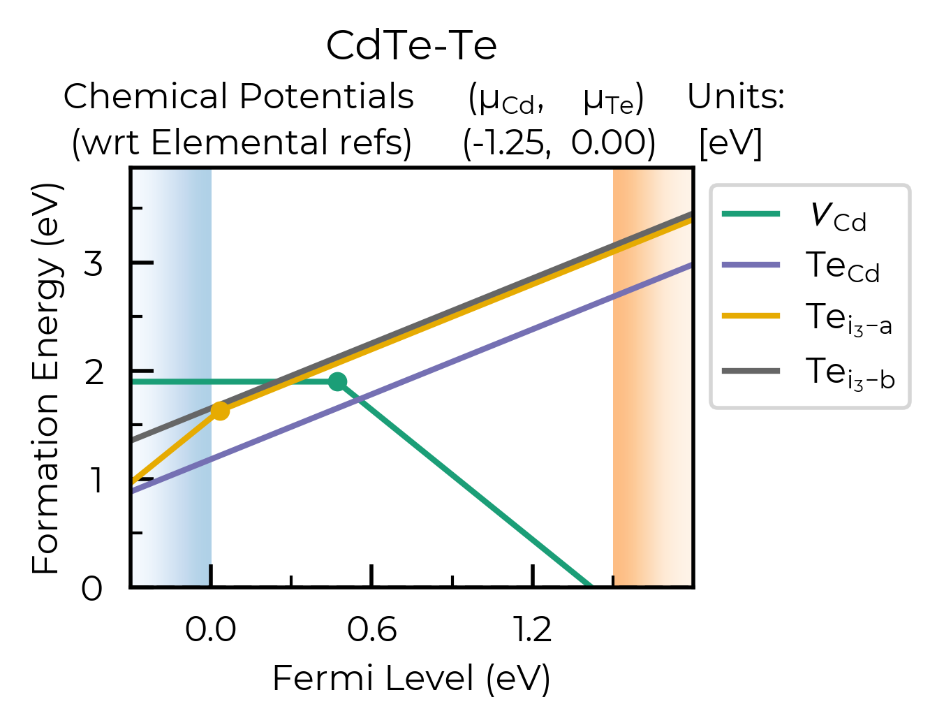
Let’s plot just the Cd vacancy defects, showing all the charge states and saving to file:

v_Cd_dpd = dpd_from_defect_dict(
    {k: v for k, v in dp.defect_dict.items() if "v_Cd" in k}
)  # only Cd vacancy defects

fig = plotting.formation_energy_plot(
    v_Cd_dpd,
    CdTe_chempots,
    auto_labels=True,
    xlim=(-0.5, 2.1),
    all_entries="faded",
    facets=["CdTe-Te"],
    filename="v_Cd_Te-Rich.pdf",
)
ax = fig.gca()
ax.axvline(0.47, ls="--", c="C4", alpha=0.4, zorder=-1)  # add a vertical line at the transition level

<matplotlib.lines.Line2D at 0x16bd28d60>

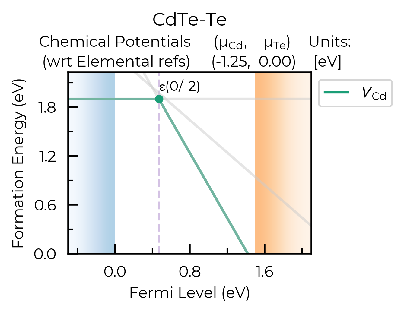
As shown here, plotting.formation_energy_plot also returns the matplotlib plot object, so you can customise this as much as you like!

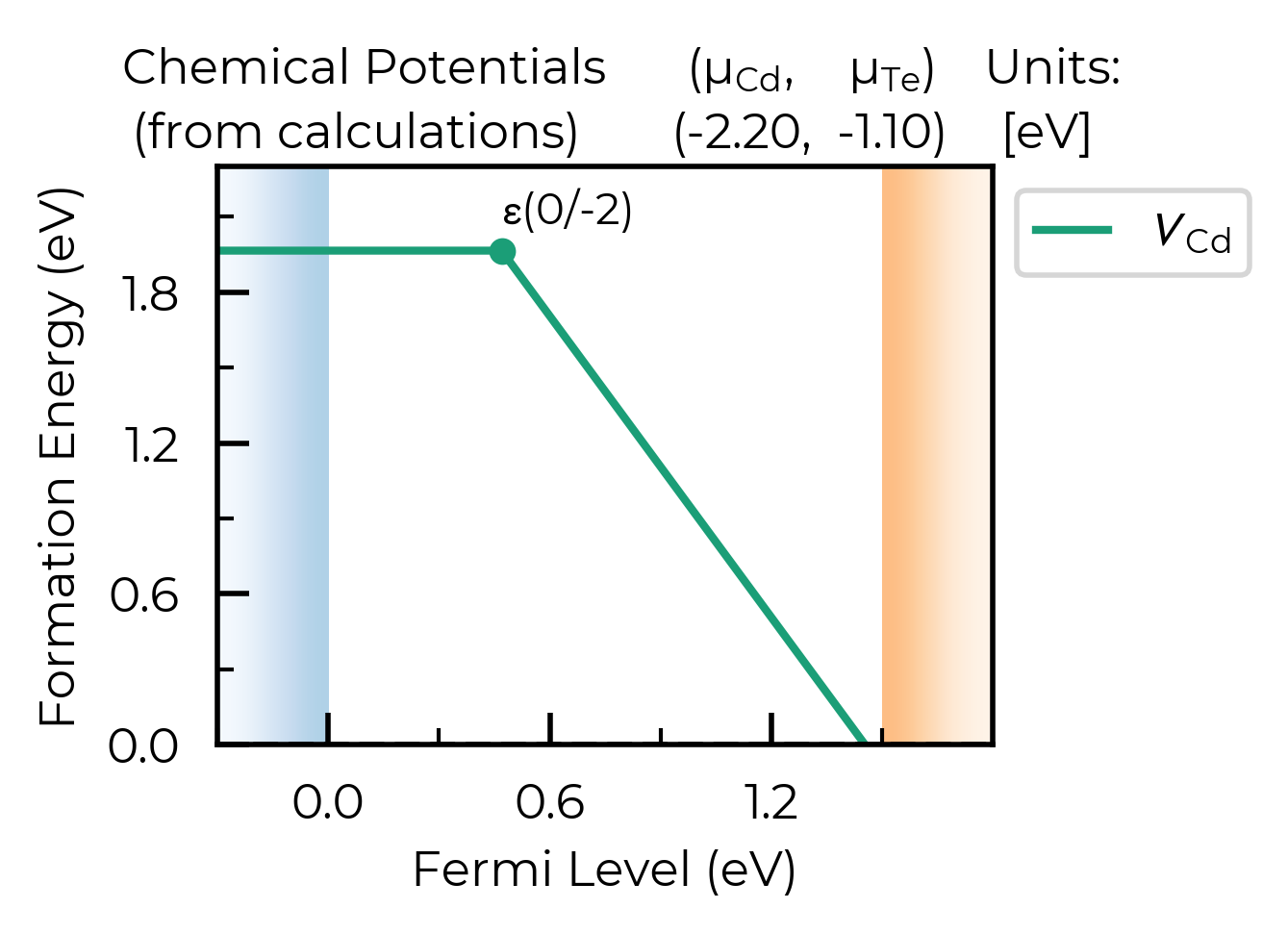
Manually inputting chemical potentials:

def_plot = plotting.formation_energy_plot(
    v_Cd_dpd,
    chempots = {"Cd": -2.2, "Te": -1.1},
    auto_labels=True,
)

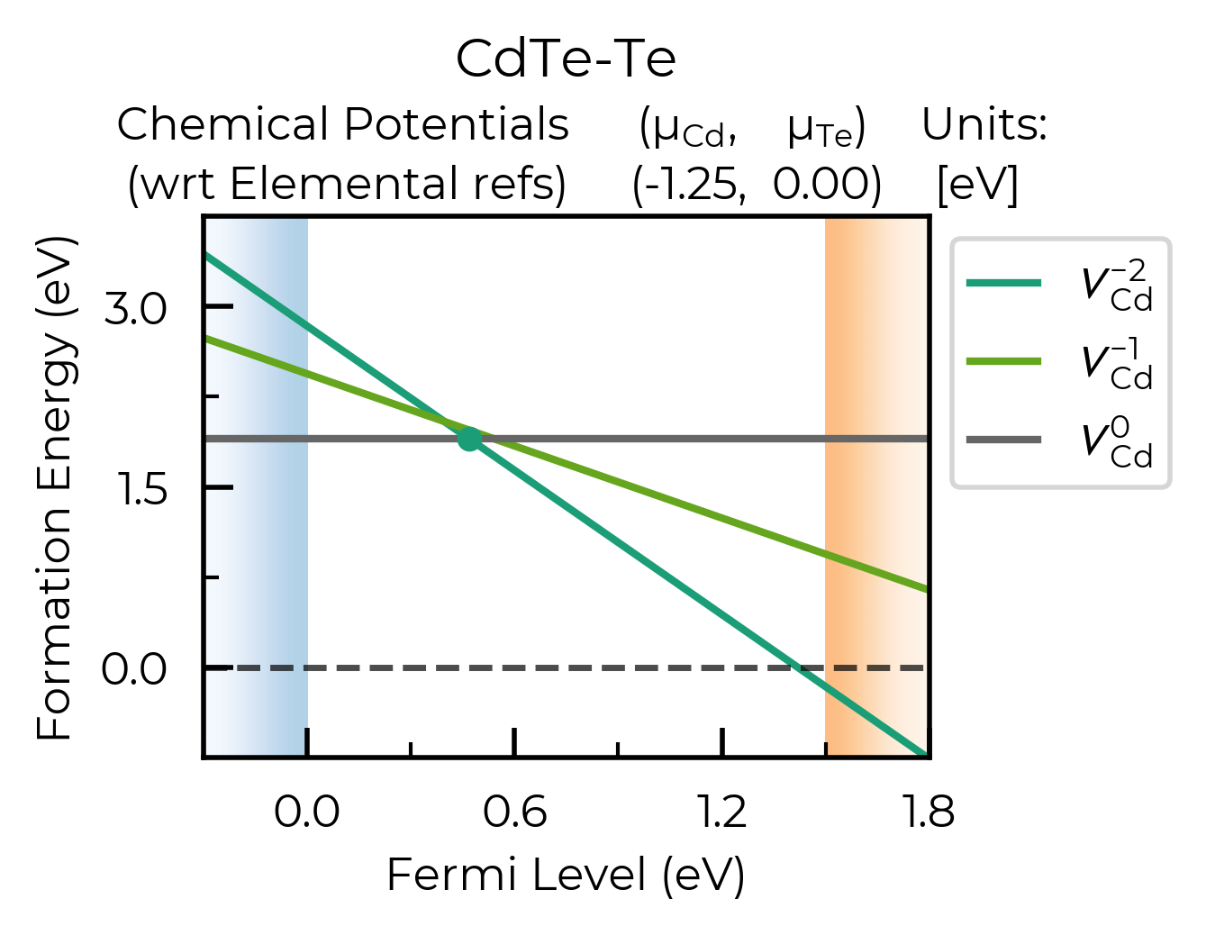
def_plot = plotting.formation_energy_plot(
    v_Cd_dpd,
    CdTe_chempots,
    all_entries=True,  # show the full formation energy lines for all defect charge states
    xlim=(-0.3, 1.8),
    ylim=(-0.75,3.75),  # adjust y-axis
    facets=["CdTe-Te"],
    filename="V_Cd_Te-Rich_All_Lines.pdf"
)

CdTe_defects_dpd = loadfn("../local_doped_testing/CdTe_FNV_dpd_for_plotting.json")

def_plot = plotting.formation_energy_plot(
    CdTe_defects_dpd,
    CdTe_chempots,
    facets=["CdTe-Te"],
)

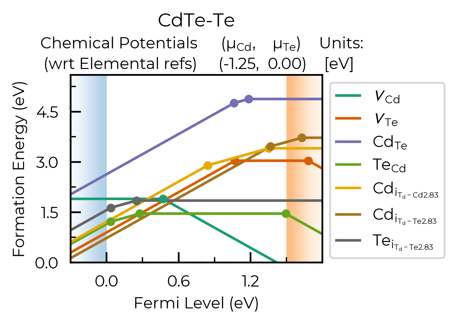
Nice! Here we can see our different inequivalent sites for the interstitials are automatically labelled in our plot legend (using the doped naming functions), showing that the lowest energy cadmium interstitial site actually differs between +2 and neutral charge states, as has been noted in this system in the literature.

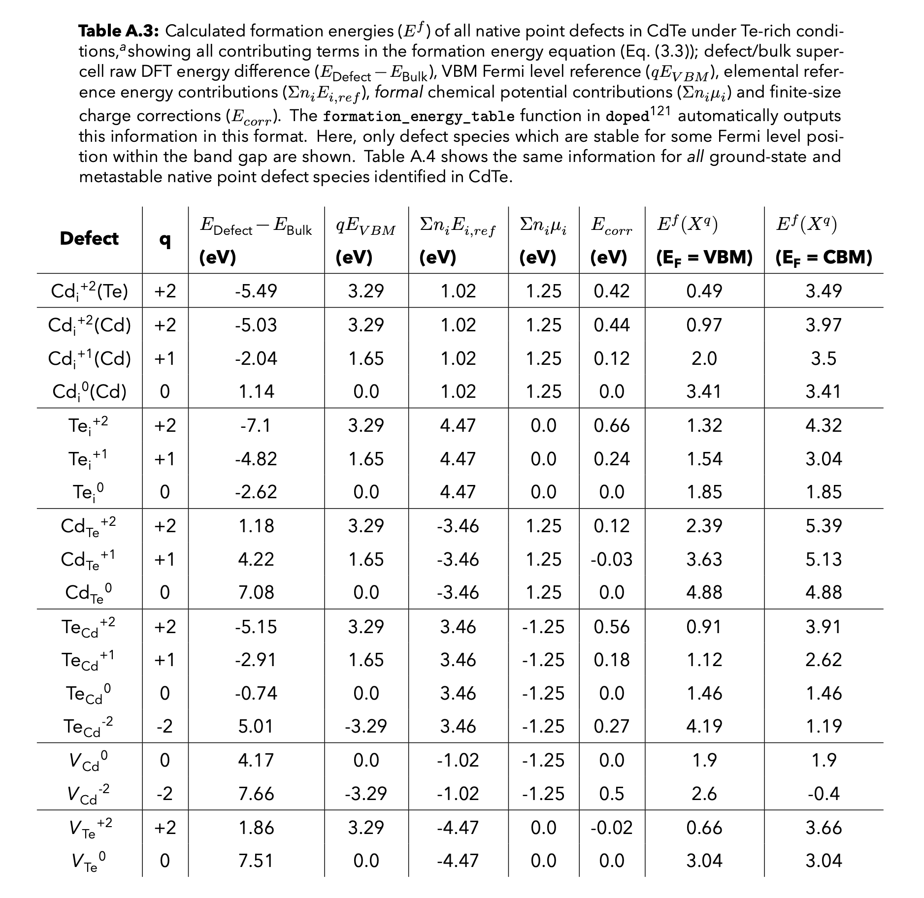
Formation Energy Tables

We can also get tables of the defect formation energies (including terms in the formation energy equation, such as the charge correction and chemical potentials), as shown below:

from doped.analysis import formation_energy_table
formation_energy_df = formation_energy_table(
    v_Cd_dpd,
    CdTe_chempots,
    facets=["CdTe-Te"],  # Te-rich facet
)
formation_energy_df

	Defect	q	ΔEʳᵃʷ	qE_VBM	qE_F	Σμ_ref	Σμ_formal	E_corr	ΔEᶠᵒʳᵐ	Path
0	v_Cd_0	0	4.166	0.000	0	-1.016	-1.251	0.000	1.899	CdTe/v_Cd_0/vasp_ncl
1	v_Cd_-1	-1	6.130	-1.646	0	-1.016	-1.251	0.225	2.441	CdTe/v_Cd_-1/vasp_ncl
2	v_Cd_-2	-2	7.661	-3.293	0	-1.016	-1.251	0.738	2.838	CdTe/v_Cd_-2/vasp_ncl

# you can run this cell to see the possible arguments for this function:
analysis.formation_energy_table?
# or go to the python API documentation for this function:
# https://doped.readthedocs.io/en/latest/doped.analysis.html#doped.analysis.formation_energy_table

Signature:
analysis.formation_energy_table(
    defect_phase_diagram: doped.utils.legacy_pmg.thermodynamics.DefectPhaseDiagram,
    chempots: Optional[Dict] = None,
    el_refs: Optional[Dict] = None,
    facets: Optional[List] = None,
    fermi_level: float = 0,
)
Docstring:
Generates defect formation energy tables (DataFrames) for either a
single chemical potential limit (i.e. phase diagram facet) or each
facet in the phase diagram (chempots dict), depending on the chempots
input supplied. This can either be a dictionary of chosen absolute/DFT
chemical potentials: {Elt: Energy} (giving a single formation energy
table) or a dictionary including the key-value pair: {"facets":
[{'facet': [chempot_dict]}]}, following the doped format. In the
latter case, a subset of facet(s) / chemical potential limit(s)
can be chosen with the facets argument, or if not specified, will
print formation energy tables for each facet in the phase diagram.

Returns the results as a pandas DataFrame or list of DataFrames.

Table Key: (all energies in eV)
'Defect' -> Defect name
'q' -> Defect charge state.
'ΔEʳᵃʷ' -> Raw DFT energy difference between defect and host supercell (E_defect - E_host).
'qE_VBM' -> Defect charge times the VBM eigenvalue (to reference the Fermi level to the VBM)
'qE_F' -> Defect charge times the Fermi level (referenced to the VBM if qE_VBM is not 0
          (if "vbm" in DefectEntry.calculation_metadata)
'Σμ_ref' -> Sum of reference energies of the elemental phases in the chemical potentials sum.
'Σμ_formal' -> Sum of _formal_ atomic chemical potential terms (Σμ_DFT = Σμ_ref + Σμ_formal).
'E_corr' -> Finite-size supercell charge correction.
'ΔEᶠᵒʳᵐ' -> Defect formation energy, with the specified chemical potentials and Fermi level.
            Equals the sum of all other terms.

Args:
    defect_phase_diagram (DefectPhaseDiagram):
        DefectPhaseDiagram for which to plot defect formation energies
        (typically created from analysis.dpd_from_defect_dict).
    chempots (dict):
        Dictionary of chemical potentials to use for calculating the defect
        formation energies. This can have the form of
        {"facets": [{'facet': [chempot_dict]}]} (the format generated by
        doped's chemical potential parsing functions (see tutorials)) and
        facet(s) (chemical potential limit(s)) to tabulate can be chosen using
        `facets`, or a dictionary of **DFT**/absolute chemical potentials
        (not formal chemical potentials!), in the format:
        {element symbol: chemical potential} - if manually specifying
        chemical potentials this way, you can set the el_refs option with
        the DFT reference energies of the elemental phases in order to show
        the formal (relative) chemical potentials as well.
        (Default: None)
    facets (list, str):
        A string or list of facet(s) (chemical potential limit(s)) for which
        to tabulate the defect formation energies, corresponding to 'facet' in
        {"facets": [{'facet': [chempot_dict]}]} (the format generated by
        doped's chemical potential parsing functions (see tutorials)). If
        not specified, will tabulate for each facet in `chempots`. (Default: None)
    el_refs (dict):
        Dictionary of elemental reference energies for the chemical potentials
        in the format:
        {element symbol: reference energy} (to determine the formal chemical
        potentials, when chempots has been manually specified as
        {element symbol: chemical potential}). Unnecessary if chempots is
        provided in format generated by doped (see tutorials).
        (Default: None)
    fermi_level (float):
        Value corresponding to the electron chemical potential. If "vbm" is
        supplied in DefectEntry.calculation_metadata, then fermi_level is
        referenced to the VBM. If "vbm" is NOT supplied in calculation_metadata,
        then fermi_level is referenced to the calculation's absolute DFT
        potential (and should include the vbm value provided by a band structure
        calculation). Default = 0 (i.e. at the VBM)

Returns:
    pandas DataFrame or list of DataFrames
File:      ~/Library/CloudStorage/OneDrive-ImperialCollegeLondon/Bread/Projects/Packages/doped/doped/analysis.py
Type:      function

Tip

The formation_energy_table function returns a list of pandas.DataFrame objects (or a single DataFrame object if a certain chemical potential facet was chosen), which we can save to csv as shown below. As a csv file, this can then be easily imported to Microsoft Word or to LaTeX (using e.g. https://www.tablesgenerator.com/latex_tables) to be included in Supporting Information of papers or in theses, which we would recommend for open-science, queryability and reproducibility!

formation_energy_df.to_csv(f"V_Cd_Formation_Energies_Te_Rich.csv", index=False)

!head V_Cd_Formation_Energies_Te_Rich.csv

Defect,q,ΔEʳᵃʷ,qE_VBM,qE_F,Σμ_ref,Σμ_formal,E_corr,ΔEᶠᵒʳᵐ,Path
v_Cd_0,0,4.166,0.0,0,-1.016,-1.251,0.0,1.899,CdTe/v_Cd_0/vasp_ncl
v_Cd_-1,-1,6.13,-1.646,0,-1.016,-1.251,0.225,2.441,CdTe/v_Cd_-1/vasp_ncl
v_Cd_-2,-2,7.661,-3.293,0,-1.016,-1.251,0.738,2.838,CdTe/v_Cd_-2/vasp_ncl

Example LaTeX table generated from the above csv file for a thesis:

Analysing Finite-Size Charge Corrections

Kumagai-Oba (eFNV) Charge Correction Example:

As mentioned above, doped can automatically compute either the Kumagai-Oba (eFNV) or Freysoldt (FNV) finite-size charge corrections, to account for the spurious image charge interactions in the defect supercell approach (see the YouTube tutorial for more details). The eFNV correction is used by default if possible (if the required OUTCAR(.gz) files are available), as it is more general – can be used for both isotropic and anisotropic systems – and the numerical implementation is more efficient, requiring smaller file sizes and running quicker.

Below, we show some examples of directly visualising the charge correction plots (showing how they are computed), which is recommended if any warnings about the charge correction accuracy are printed when parsing our defects (also useful for understanding how the corrections are performed!).

Here we’re taking the example of a Fluorine-on-Oxygen antisite substitution defect in Y₂Ti₂O₅S₂ (a potential photocatalyst and n-type thermoelectric), which has a non-cubic anisotropic structure and dielectric constant:

from doped.analysis import DefectParser  # can use DefectParser to parse individual defects if desired
F_O_1_entry = DefectParser.from_paths(defect_path="YTOS/F_O_1", bulk_path="YTOS/Bulk",
                                                dielectric = [40.7, 40.7, 25.2]).defect_entry
print(f"Charge: {F_O_1_entry.charge_state:+} at site: {F_O_1_entry.defect_supercell_site.frac_coords}")
print(f"Finite-size charge corrections: {F_O_1_entry.corrections}")

Charge: +1 at site: [0. 0. 0.]
Finite-size charge corrections: {'kumagai_charge_correction': 0.12691248591191384}

Above, the defect has been parsed and the anisotropic (eFNV) charge correction correctly applied, with no warnings thrown. We can directly plot the atomic site potentials which are used to compute this charge correction if we want: (Though typically we only do this if there has been some warning or error related to the application of the defect charge correction – here we’re just showing as a demonstration)

Note

Typically we only analyze the charge correction plots like this if there has been some warning or error related to the defect charge correction (or to aid our understanding of the underlying formation energy calculations). Here we’re just showing as a demonstration.

correction, plot = F_O_1_entry.get_kumagai_correction(plot=True)

Calculated Kumagai (eFNV) correction is 0.127 eV

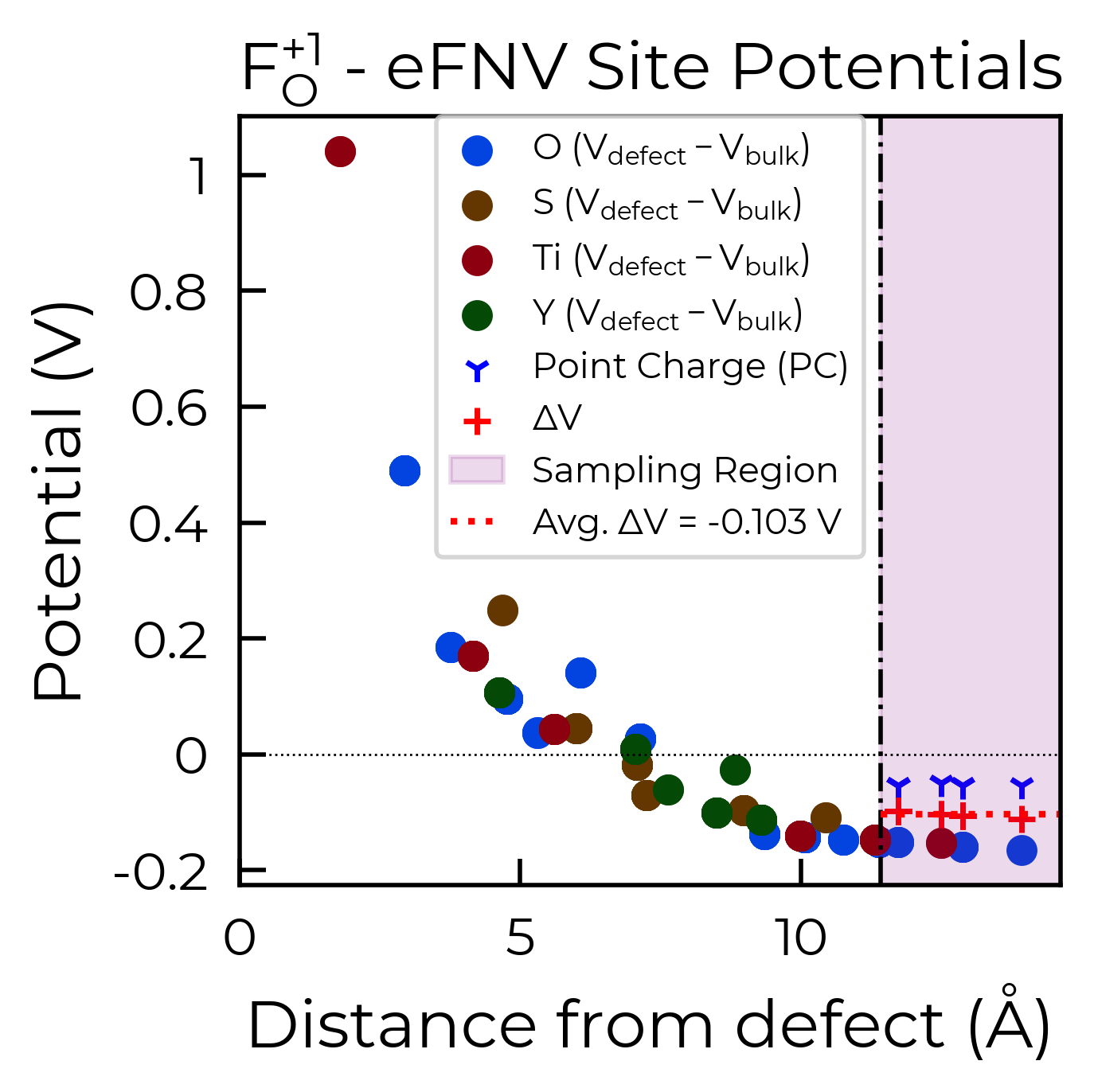
Here we can see we obtain a good plateau in the atomic potential differences (ΔV) between the defect and bulk supercells in the ‘sampling region’ (i.e. region of defect supercell furthest from the defect site), the average of which is used to obtain our potential alignment (‘Avg. ΔV’) and thus our final charge correction term.

If there is still significant variance in the site potential differences in the sampling region (i.e. a converged plateau is not obtained), then this suggests that the charge correction may not be as accurate for that particular defect or supercell. This error range of the charge correction is automatically computed by doped, and can be returned using the return_correction_error argument in get_kumagai_correction/get_freysoldt_correction, or also by adjusting the error_tolerance argument:

correction = F_O_1_entry.get_kumagai_correction(error_tolerance=0.0001)  # extremely strict tolerance, 0.1 meV

Calculated Kumagai (eFNV) correction is 0.127 eV

core.py:215: UserWarning: Estimated error in the Kumagai (eFNV) charge correction for defect F_O_1 is 0.001 eV (i.e. which is than the `error_tolerance`: 0.000 eV). You may want to check the accuracy of the correction by plotting the site potential differences (using `defect_entry.get_kumagai_correction()` with `plot=True`). Large errors are often due to unstable or shallow defect charge states (which can't be accurately modelled with the supercell approach). If this error is not acceptable, you may need to use a larger supercell for more accurate energies.

correction, error = F_O_1_entry.get_kumagai_correction(return_correction_error=True)
error  # calculated error range of 1.3 meV in our charge correction here

Calculated Kumagai (eFNV) correction is 0.127 eV

0.0013276476471274629

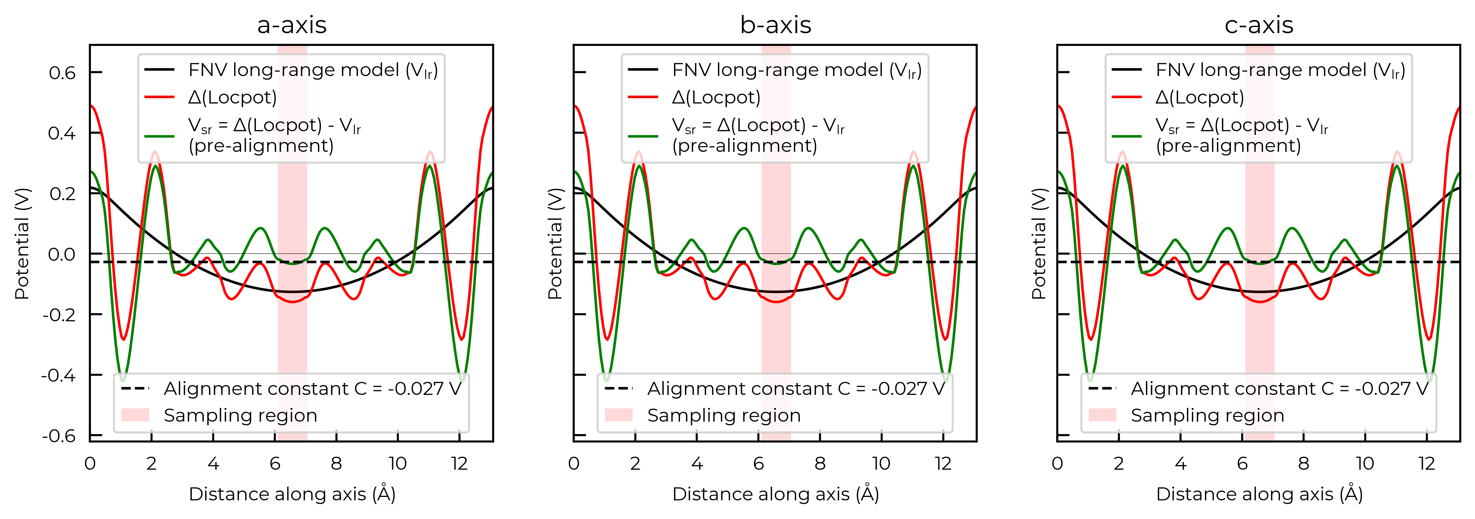
Freysoldt (FNV) Charge Correction Example:

Above, we used the Kumagai-Oba (eFNV) defect image charge correction scheme, which is compatible only with both isotropic and anisotropic dielectric screening.

doped also supports the original Freysoldt (FNV) charge correction scheme, however this should only be used for isotropic/cubic host materials (and even then the eFNV correction is still preferred, being more efficient and robust in implementation). For the FNV correction, the LOCPOT(.gz) output files must be present in our defect and bulk supercell calculation directories.

correction, plot = CdTe_defect_dict["v_Cd_-2"].get_freysoldt_correction(plot=True)

Calculated Freysoldt (FNV) correction is 0.738 eV

Further Defect Analysis

As briefly discussed in the YouTube defects tutorial, you will likely want to further analyse the key defect species in your material, by e.g. visualising the relaxed structures with VESTA/CrystalMaker, looking at the defect single-particle energy levels using the sumo DOS plotting functions (sumo-dosplot), charge density distributions (e.g. this Figure).

In particular, you may want to further analyse the behaviour and impact on material properties of your defects using advanced defect analysis codes such as py-sc-fermi (to analyse defect concentrations, doping and Fermi level tuning), easyunfold (to analyse the electronic structure of defects in your material), or nonrad / CarrierCapture.jl (to analyse non-radiative electron-hole recombination at defects). The outputs from doped are readily ported as inputs to these codes.

Further Post-Processing and Correction Analysis

Here we describe some more targeted analysis you can do for your defect calculations (including comparing the relaxed configurations for different initial interstitial positions, structure & bond length analysis of defects, and plotting/analysis of the defect charge corrections), which may be useful for in certain cases.

Processing Cdᵢ vasp_gam calculations to see which site is favoured

import os

bulk_path = "CdTe/CdTe_bulk/vasp_gam/"  # path to bulk (defect-free) supercell calculation
dielectric = 9.13  # calculated dielectric constant, required for computing defect charge corrections
Cd_i_dict = {}  # Keep dictionary of parsed defect entries

for i in os.listdir("CdTe"):
    if 'Cd_i' in i:
        Cd_i_dict[i] = DefectParser.from_paths(
            defect_path=f"CdTe/{i}/vasp_gam/", bulk_path=bulk_path, dielectric=dielectric).defect_entry

for defect_name, defect_entry in Cd_i_dict.items():
    print(f"Name: {defect_name}; Raw Supercell Energy: {defect_entry.get_ediff():.3f} eV")
    # note this energy is just the energy difference of the bulk and defect supercells (including 
    # finite-size charge corrections if any – none here as they're neutral defects), without Fermi
    # level or chemical potential terms (though these are constant for the same defect & charge)

Name: Cd_i_Td_Cd2.83_0; Raw Supercell Energy: 0.592 eV
Name: Cd_i_C3v_0; Raw Supercell Energy: 0.728 eV
Name: Cd_i_Td_Te2.83_0; Raw Supercell Energy: 0.728 eV

Here we see that the Cd-coordinated interstitial site is the lowest energy for neutral cadmium interstitials here!

Note

The energies here do not yet account for the chemical potentials, which are included later in the post-processing workflow (as shown earlier in this notebook). However, the chemical potential energy correction is the same for each charge state or site, for a given defect (e.g. Cd_i here) - hence the relative energies are still meaningful here.

Here we see that Cd_i_C3v_0 and Cd_i_Td_Te2.83_0 have equal final energies (rounded to 1 meV/atom) suggesting they have relaxed to the same final structure (despite different initial interstitial positions). Let’s use StructureMatcher and local_env to double-check:

# Here we use the pymatgen StructureMatcher class to compare the relaxed structures of neutral Cd_i:
from pymatgen.analysis.structure_matcher import StructureMatcher
sm = StructureMatcher()
print("Are Cd_i_Td_Cd2.83_0 and Cd_i_C3v_0 final structures the same?:",
      sm.fit(Cd_i_dict['Cd_i_Td_Cd2.83_0'].defect_supercell, Cd_i_dict['Cd_i_C3v_0'].defect_supercell))
print("Are Cd_i_C3v_0 and Cd_i_Td_Te2.83_0 final structures the same?:",
      sm.fit(Cd_i_dict['Cd_i_C3v_0'].defect_supercell, Cd_i_dict['Cd_i_Td_Te2.83_0'].defect_supercell))

Are Cd_i_Td_Cd2.83_0 and Cd_i_C3v_0 final structures the same?: False
Are Cd_i_C3v_0 and Cd_i_Td_Te2.83_0 final structures the same?: True

# we can perform further defect structural analysis with these functions:
from pymatgen.analysis.local_env import CrystalNN
import numpy as np

for key, defect_entry in Cd_i_dict.items():
    # get defect site index in structure: (needed for CrystalNN)
    for i, site in enumerate(defect_entry.defect_supercell.sites):
        if np.isclose(site.frac_coords, defect_entry.defect_supercell_site.frac_coords).all():
            isite = i  # site index, starting from 0

    crystalNN = CrystalNN()
    struct = defect_entry.defect_supercell
    struct.add_oxidation_state_by_guess()
    print("Local order parameters (i.e. resemblence to given structural motif): ",
          crystalNN.get_local_order_parameters(struct, isite))
    print("Nearest-neighbour dictionary: ",
          crystalNN.get_cn_dict(struct, isite))

    bond_lengths = []  # Bond Lengths?
    for i in crystalNN.get_nn_info(struct, isite):
        bond_lengths.append({'Element': i['site'].specie.as_dict()['element'],
                             'Distance': f"{i['site'].distance(struct[isite]):.3f}"})
    print("Bond-lengths (in Angstrom) to nearest neighbours: ", bond_lengths, "\n")

Local order parameters (i.e. resemblence to given structural motif):  None
Nearest-neighbour dictionary:  {'Te0+': 6, 'Cd0+': 4}
Bond-lengths (in Angstrom) to nearest neighbours:  [{'Element': 'Te', 'Distance': '3.298'}, {'Element': 'Te', 'Distance': '3.298'}, {'Element': 'Te', 'Distance': '3.298'}, {'Element': 'Te', 'Distance': '3.298'}, {'Element': 'Te', 'Distance': '3.298'}, {'Element': 'Te', 'Distance': '3.298'}, {'Element': 'Cd', 'Distance': '3.007'}, {'Element': 'Cd', 'Distance': '3.007'}, {'Element': 'Cd', 'Distance': '3.007'}, {'Element': 'Cd', 'Distance': '3.007'}] 

Local order parameters (i.e. resemblence to given structural motif):  {'square co-planar': 0.08049643519922586, 'tetrahedral': 0.9999935468913711, 'rectangular see-saw-like': 0.007133072179242341, 'see-saw-like': 0.23547633536015408, 'trigonal pyramidal': 0.24644908542744104}
Nearest-neighbour dictionary:  {'Te0+': 4}
Bond-lengths (in Angstrom) to nearest neighbours:  [{'Element': 'Te', 'Distance': '2.911'}, {'Element': 'Te', 'Distance': '2.911'}, {'Element': 'Te', 'Distance': '2.911'}, {'Element': 'Te', 'Distance': '2.911'}] 

Local order parameters (i.e. resemblence to given structural motif):  {'square co-planar': 0.07996844283674677, 'tetrahedral': 0.9999999999971609, 'rectangular see-saw-like': 0.0070246315480141, 'see-saw-like': 0.23425410407519495, 'trigonal pyramidal': 0.2452100857961308}
Nearest-neighbour dictionary:  {'Te0+': 4}
Bond-lengths (in Angstrom) to nearest neighbours:  [{'Element': 'Te', 'Distance': '2.911'}, {'Element': 'Te', 'Distance': '2.911'}, {'Element': 'Te', 'Distance': '2.911'}, {'Element': 'Te', 'Distance': '2.911'}] 

Here we see the structural similarity of “Cd_i_C3v_0” and “Cd_i_Td_Te2.83_0”, showing that they have indeed relaxed to the same structure. This means we only need to continue with one of these for the more expensive vasp_std and vasp_ncl calculations with our full k-point mesh.

Note

If you want to do this coordination environment analysis with a vacancy, you may have to introduce a fake atom at the vacancy position, in order to create a pymatgen Site object, to then use with CrystalNN. For example:

from pymatgen.analysis.local_env import CrystalNN
from doped import analysis

for defect_entry in v_Cd_dpd.entries:
    analysis.bold_print(f"{defect_entry.name}, Charge State: {defect_entry.charge_state}")
    crystalNN = CrystalNN(distance_cutoffs=None, x_diff_weight=0.0, porous_adjustment=False, search_cutoff=5)
    struct = defect_entry.defect_supercell.copy()
    struct.append('U', defect_entry.defect_supercell_site.frac_coords) # Add a fake element
    isite = len(struct.sites) - 1 # Starts counting from zero!

    print("Local order parameters (i.e. resemblance to given structural motif): ",
          crystalNN.get_local_order_parameters(struct, isite))
    print("Nearest-neighbour dictionary: ", crystalNN.get_cn_dict(struct, isite))

    bond_lengths = []  # Bond Lengths?
    for i in crystalNN.get_nn_info(struct,isite):
        bond_lengths.append({'Element': i['site'].specie.as_dict()['element'],
                             'Distance': f"{i['site'].distance(struct[isite]):.3f}"})
    print("Bond-lengths (in Angstrom) to nearest neighbours: ",bond_lengths,"\n")

v_Cd_0, Charge State: 0
Local order parameters (i.e. resemblance to given structural motif):  {'square co-planar': 0.1554382566688805, 'tetrahedral': 0.7810051379511412, 'rectangular see-saw-like': 0.052869064285435134, 'see-saw-like': 0.22758740109965894, 'trigonal pyramidal': 0.23528866099223875}
Nearest-neighbour dictionary:  {'Te': 4}
Bond-lengths (in Angstrom) to nearest neighbours:  [{'Element': 'Te', 'Distance': '2.178'}, {'Element': 'Te', 'Distance': '2.605'}, {'Element': 'Te', 'Distance': '2.235'}, {'Element': 'Te', 'Distance': '2.671'}] 

v_Cd_-1, Charge State: -1
Local order parameters (i.e. resemblance to given structural motif):  {'square co-planar': 0.08955199275710107, 'tetrahedral': 0.9980437792997895, 'rectangular see-saw-like': 0.00914205834683717, 'see-saw-like': 0.2561471898083992, 'trigonal pyramidal': 0.2673736880526364}
Nearest-neighbour dictionary:  {'Te': 4}
Bond-lengths (in Angstrom) to nearest neighbours:  [{'Element': 'Te', 'Distance': '2.585'}, {'Element': 'Te', 'Distance': '2.587'}, {'Element': 'Te', 'Distance': '2.587'}, {'Element': 'Te', 'Distance': '3.046'}] 

v_Cd_-2, Charge State: -2
Local order parameters (i.e. resemblance to given structural motif):  {'square co-planar': 0.07996848894580866, 'tetrahedral': 0.999999999996243, 'rectangular see-saw-like': 0.007024644113827354, 'see-saw-like': 0.23425369905750856, 'trigonal pyramidal': 0.24520967518806777}
Nearest-neighbour dictionary:  {'Te': 4}
Bond-lengths (in Angstrom) to nearest neighbours:  [{'Element': 'Te', 'Distance': '2.613'}, {'Element': 'Te', 'Distance': '2.613'}, {'Element': 'Te', 'Distance': '2.613'}, {'Element': 'Te', 'Distance': '2.613'}]